Download
1 / 27
270 likes | 417 Views
EXAMPLE OF MARINE MODELING Seafloor stratigraphy and its variability: a numerical modeling approach. Irina Overeem and James Syvitski Environmental Computation and Imaging Facility INSTAAR, University of Colorado, Boulder, CO. Objectives.

E N D
EXAMPLE OF MARINE MODELINGSeafloor stratigraphy and its variability: a numerical modeling approach Irina Overeem and James Syvitski Environmental Computation and Imaging Facility INSTAAR, University of Colorado, Boulder, CO
Objectives • Develop an expert system for determination of environmental boundary conditions and their time-variability on a global scale. These boundary conditions are input to the stratigraphic simulation models. • Characterization of sea floor and shallow shelf stratigraphy with HydroTrend and 2D-SedFlux numerical modeling and test model predictions against observed sea floor data. • Determine sea floor variability by running 2D-SedFlux sensitivity tests • Develop measures and visualization that quantify model prediction uncertainty New Jersey shelf stratigraphy is used as the case-study to illustrate the research results.
2DSedFlux INPUT(t) sea level(t), bathymetry (t-0) Q, Qs, Qb PROCESSES River: avulsion, floodplain SR Marine: delta plume, stormreworking Basin: compaction • OUTPUT (x,z,t) • 2D-geometry • grain size, permeability, bulk density, porosity Numerical models: Hydrotrend and SedFlux HydroTrend INPUT(t) T, P, A, H, ELA + statistical properties PROCESSES Hydrological mass balance (daily) Qi =Qsurf +Qniv + Qgw+Qice Empirical relation Qs ~ A, H, T Qs ~ ψ (Qi /Qmean)c OUTPUT (t) - Q, Qs, Qb (daily) for 5 grain-size classes
I Expert system for retrieval of time-continuous environmental conditions • The present-day sea floor and shallow stratigraphy is determined by changing depositional processes over time, often recording 1000’s of years of evolution. The depositional processes are controlled by longterm sea-level changes and climate changes (like temperature and precipitation patterns, storm climate and sea-ice or glacial melt). • Estimates of environmental conditions are now being retrieved from global datasets and environmental models (e.g Community Climate System Models) for our stratigraphic modeling purposes. • Interpolation schemes have been developed to reconstruct time-continuous signals between observed data (mostly >100 yrs) and time-slices of paleo-data from environmental numerical models. Continuous proxy records, like δO18 in deep marine cores or dust in Greenland ice cores, are used to drive the relative changes over time.
Sea level and Ice Sheet evolution Digital Elevation Models (GTOPO30) and global bathymetric data sets have been integrated with a global sea-level curve and Laurentide Ice Sheet predictions to make quantitative assessment of US East Coast drainage basin characteristics over time possible. Time slices at 40ka, 21ka, 12ka and the present for the Hudson River basin are shown.
Community Climate System Model (CCM1) Predicts daily statistics of global temperature and precipitation at time slices in past (21 kBP, 18kBP, 16kBP, 12kBP, 8kBP). CCM1 predicted global monthly changes in temperature at 21ka are shown. Glaciological Model (ICE4G) Predicts global Ice Cap melt from 21kBP to present-day (Peltier et al., 1994), which provides glacier dynamics and meltwater discharges to HydroTrend
Boundary Conditions: River Sediment HydroTrend predicts river sediment load, Qs over time as function of: • A, R = Area and relief are drainage basin characteristics retrieved from integrated Digital Elevation Models and bathymetry. • P, T = Precipitation and temperature retrieved from climate stations and Community Climate Model paleo-realizations (CCM1), interpolated with climate proxies • Qice = Ice melt retrieved from glaciological models • TE = Sediment trapping efficiency based on lake areas in basin • α, k = Empirical coefficients (Syvitski et al., 2003). larger uncertainty smaller uncertainty
Boundary Conditions: Storm Climate • WAVE-WATCH III provides global wave climate, (3hr time intervals) • Use the significant wave height (H) • to set SedFlux log-normal wave height distribution use the peak month • offshore NJ this would be 7.2 m
Boundary Conditions: Initial bathymetric profile Hudson River 2D-SedFlux simulation corridor The initial bathymetric profile can be synthesized with high uncertainty from the present bathymetry. Local seismic information potentially has a higher accuracy. The New Jersey SedFlux simulation used an evident regional reflector as an initial surface (‘R’-reflector based on seismic data interpretations by Goff & Gulick, UTA)
Conclusions (I) • High-resolution environmental variables and their associated variability are increasingly online available on global scale, which makes SedFlux seafloor predictions possible in data-sparse areas. • The uncertainty in these environmental variables is significant; an order of magnitude range is not unusual. • The uncertainty in the boundary conditions increases rapidly with larger time scales over the geological history, this inherently influences the performance of SedFlux with increasing depth below the seabed. Without accurate records for the environmental variables, it is unlikely that the model predictions will be accurate. • This suggests that SedFlux-2D may be most successful in predicting the acoustic properties of sediments that have been deposited over the past century or more in regions of high sediment accumulation (e.g., offshore of major rivers) and for which there are well-documented records of sediment input, waves and currents.
SedFlux simulation of 40,000 years of shelf deposition: line 910
SedFlux simulation of 40,000 years of shelf deposition: line 907
SedFlux predicted properties - grain size, bulk density, porosity, permeability per 10 cm bin - volume fraction per grainsize
II Testing SedFlux against observed data FIRST-ORDER TEST • High resolution seismic data interpretation: mapped the thickness of sediment above the R-reflector • 98 seafloor grab samples, GeoClutter dataset (grain size) (Goff et al, 2003). • dbSEABED (Jenkins, INSTAAR), usSEABED (Williams, USGS). BLIND TEST (Pratson, Duke; Kraft, UNH; Holland, Penn State) • Acoustic scatter measurements • Low grazing angle seismic experiments (7 stations)
Shallow Stratigraphy Seismic reconstruction of Chirp sonar & 2D Huntec data, (after Duncan et al, 2000). Simulation shows a sea-level-rise controlled retrograding system. Late Pleistocene deposition is high and leaves an extensive deltaic wedge close to the shelf slope at 110 km. Intense storm reworking moves the depocenter of the delta to ~160 m water depth. A large part of the shallow shelf has only a thin veneer of sediment. The yellow colors represent coarse fluvial sediment and near-coastal zone sands. Over the last 10k, sea level rise slows down. The wedge is much less extensive though, because the river contributes less sediment after the decoupling of the large ice-sheet drainage.
Large-scale layer geometry Red and green lines show the deposited sediment thickness over the entire SedFlux simulation against water depth. The 3D interpreted surface of the R-reflector depth is collapsed into a mean thickness of sediments above the R-reflector per water depth (blue line). The predicted SedFlux thickness matches the observed thickness rather closely and falls for the greater part well within the observed range (dotted blue lines).
Grab Sample Locations 98 grab samples taken in the 2001 with Smith-McIntyre grab sampler (sampling size 500-1000g), between 50 -150m water depth (Goff et al., 2003) Grain size data based on 556 sea floor samples between 40-160 m water depth over a wider zone on the New Jersey margin (-74.5 to -71.5 lat, 41.5 to 38.5 long) from the dbSeaBed system. (Jenkins, 1997; Williams et al., 2003).
Seafloor grain size Comparison of grain size data against the SedFlux prediction the uppermost two bins (0 – 20 cm). The dbSeaBed data set covering a wide zone on the New Jersey margin shows how laterally variable the grain sizes are. It is clear from both observed data sets that coarse sand occurs in 120 to 140 m water depth. SedFlux shows a larger component of fine sand. Exceptionally coarse samples in observed data are not matched by SedFlux, because initial grain-size distribution of the SedFlux simulations did not include gravels, nor biogenic material. SedFlux predicts the grain size well within the range of the observed values, although with an overprediction of fine sediment.
Conclusions (II) • SedFlux simulation reasonably predicts the observed stratigraphic pattern. The thickness and location of the predicted sediment wedges compares well with observations. The SedFlux prediction is well within the observed range of thicknesses over the shallow shelf. • A veneer of terrestrial fluvial sediments of Late Pleistocene age is predicted to occur close to the present-day seafloor surface. The acoustically observed channels are not explicitly matched in the SedFlux prediction, since SedFlux-2D can not reproduce distinct channels. However, the predicted coarse fluvial sediment is the typical facies that would contain channel bodies in a three-dimensional model. • SedFlux predicts the grain size at the sea floor approximately in the range of the observed values, although with a consistent overprediction of fine sediment. The initial grain-size distribution of the SedFlux simulations did not include gravels or biogenic material, so occurrences of gravels or abundant shell hash are not accounted for in the modeling.
III Seafloor variability • In the process of reconstructing the boundary conditions the uncertainty in the estimates is evident. The ranges of uncertainty in the boundary conditions impose a series of sensitivity tests. The tests have 20% range in the environmental boundary conditions. • Sensitivity tests are compared to weigh the influence of specific environmental parameters with the use of the L2-norm. The deviation of the sensitivity test (ST) from the base case simulation (BC) is expressed as: thickness distribution (TH) grain size (GSD) • 16 sensitivity tests are associated with the ‘base-case’ to provide us with an idea of sea floor variability.
Sensitivity tests example: strong influence of initial profiles • Influence of initial profile • initial slope influences the spreading width of the deposited wedges over the shelf • local irregularities are being filled in and leave uniquely shaped deposits (like in the zoom-in part of line 910) • general stratigraphy and the distribution of distinct grain sizes remains similar
Sensitivity test example: strong influence of storm climate • Storm climate is shown to have important effects on both the geometry and the grain-size prediction in the topmost layer. More intense storm climate moves fine sediments to deeper water, in that way shifting the locations of the depocenters • This sensitivity test which simulates no storms at all, deviates so strongly from the observed coarse grain size at the sea floor that it could be disregarded for that reason.
Sensitivity test example: little influence of changing sea level curve We postulated that the New Jersey margin probably had undergone considerable isostatic movement due to unloading of the Laurentide Ice sheet. Surprisingly, the use of a global sea level curve (green line) or a local sea level curve, which incorporates isostatic tectonic movements, (red line), is shown to have little effects on the large-scale predicted geometry.
Intercomparison of Sensitivity tests with L2-norm The L2 norm values show that the SedFlux predictions of both the thickness distribution as well as the topmost grain-size distribution are the most sensitive to uncertainty in the ocean storm climate. Among the environmental parameters influencing sediment supply (drainage area, precipitation, and temperature), elevation (R) stands out as the factor that has the strongest relative impact on the predicted properties.Uncertainty in the drainage area characteristics would thus affect the prediction as well.
Conclusions (III) • L2 norm is a successful measure to quantify the sensitivity of the SedFlux model prediction to specific environmental parameters. • Storm climate has high uncertainty (especially for the reconstructions of past conditions). In addition, the SedFlux grain size predictions have high sensitivity for changes in the storm climate. • Some environmental parameters do not have such strong impact on the SedFlux predictions in the analysis of the sensitivity tests. Note however that most parameters influencing the sediment supply (drainage area, precipitation and temperature) could have potentially higher uncertainty than the 20% range used for the assessment. • SedFlux provides a method to quantify variability due to uncertainties in the boundary conditions by running different input scenarios = sensitivity tests.
Publications • Hutton, E.W.H. and Syvitski, J.P.M., 2003. Advances in the Numerical Modeling of Sediment Failure during the development of a continental margin. Marine Geology, 203: 367-380. [published, refereed] • Morehead, M., Syvitski, J.P.M, Hutton, E.W.H., and Peckham, S.D., 2003. Modeling the interannual and intra-annual variability in the flux of sediment in ungauged river basins. Global and Planetary Change, 39: 95-110. • Overeem, I. Syvitski, J.P.M., Hutton, E.W.H., Kettner, A.J. 2004. Stratigraphic variability due to uncertainty in model boundary conditions: a case-study of the New Jersey Shelf over the last 40,000 years. Marine Geology • Syvitski, J.P.M. and Hutton, E.W.H., 2003. Failure of marine deposits and their redistribution by sediment gravity flows. Pure and Applied Geophysics,160: 2053-2069. [published, refereed] • Kraft, B.J., Overeem, I., Holland, C.W., Pratson, L.F., Syvitski, J.P.M. , Mayer, L.A., 2004. Stratigraphic model predictions of geoacoustic properties. Journal of Ocean engineering.