Download
1 / 25
250 likes | 340 Views
Estimation of daily CO 2 fluxes over Europe by inversion of atmospheric continuous data. C. Carouge and P. Peylin ; P. Bousquet ; P. Ciais ; P. Rayner. Laboratoire des Sciences du Climat et de l’Environnement. Acknowledgement : all experimentalists from Aerocarb project.

E N D
Estimation of daily CO2 fluxes over Europe by inversion of atmospheric continuous data C. Carouge and P. Peylin ; P. Bousquet ; P. Ciais ; P. Rayner Laboratoire des Sciences du Climat et de l’Environnement Acknowledgement : all experimentalists from Aerocarb project
How to assimilate daily measurements ? Schauinsland CO2 (ppm) high spatial resol. Model daily time step inversion
Inversion setup • Period :1 year = 2001 • Observations :10 European stations, daily averaged data • Transport model :LMDZ, zoom over Europe • Fluxes :- Europe & North east Atlantic : each pixel / daily • - Elsewhere : subcontinental regions / monthly • Prior :Fluxes : optimised monthly fluxes • Errors : 1 GtC/year over Europe • 0.5 GtC/year over north east Atlantic • tiny on other regions • Correlations :spatial and temporal variable correlationsbetween European pixels
Continuous European measurement sites Continuous sites AEROCARB data base : http://www.aerocarb.cnrs-gif.fr/database.html
Inversion setup • Period :1 year = 2001 • Observations :10 European stations,daily averaged data • Transport model :LMDZ, zoom over Europe • Fluxes :- Europe & North east Atlantic : each pixel / daily • - Elsewhere : subcontinental regions / monthly • Prior :Fluxes : optimised monthly fluxes • Errors : 1 GtC/year over Europe • 0.5 GtC/year over north east Atlantic • tiny on other regions • Correlations :spatial and temporal variable correlationsbetween European pixels
Transport model • 192 x 146 and 19 vertical levels-0.5 x 0.5 degrees in the zoom • - 4 x 4 degrees at the lowest resolution • Nudged on ECMWF winds
Inversion setup • Period :1 year = 2001 • Observations :10 European stations,daily averaged data • Transport model :LMDZ, zoom over Europe • Fluxes :- Europe & North east Atlantic : each pixel / daily • - Elsewhere : subcontinental regions / monthly • Prior : Fluxes : pre-optimised monthly fluxes • Errors : 1 GtC/year over Europe • 0.5 GtC/year over north east Atlantic • tiny on other regions • Correlations :spatial and temporal correlations between European / N.Atlantic pixels
Spatial and temporal correlations Based on correlation lengths: Distance(i,j) : distance in space or time between 2 fluxes i, j • L spatial : 500 - 800 km • L temporal : 5 – 15 days
Technical aspects : • Use “retro-plume approach” (~ adjoint) to get daily response functions for all pixels • Two steps inversion : - 1st : standard monthly Fluxes + Globalview data- 2nd : daily fluxes using the 1st step estimated fluxes.. • Synthesis inversion to get posterior errors : Huge memory size problems ! Sequential approach with overlap : 11 * 2 months inversions Still 7000*60 unknowns covariance matrix of ~ 400,000 x 400,000 !!
FIRST RESULTS ( Still preliminary)
Two different inversions First inversion • 10 sites : Cabauw tower at 120m and 200m • Data : full daily mean • Data-error : stdev of hourly measurements • Time correlation length : 5 days • Spatial correlation lengths : 500/800 Km for land/ocean Updated inversion • 9 sites : Cabauw tower at 200 m + data-error x 3 in winter • Data : daytime-only mean • Time correlation : 15 days
Fit to the stations : Westerland Observations + error bars Posterior Prior 16/01 22/03 27/05 3/08 22/10 15/12 (Days)
Fit to the stations : Monte Cimone Observations + error bars Posterior Prior 16/01 22/03 27/05 3/08 22/10 15/12 (Days)
Aerocarb project : Forward simulation with REMOD model Diurnal cycle At Monte-Cimone “Proper” vertical level (appropriated in winter) Need to use different levels depending on the season
Fit to the stations : Schauinsland Observations + error bars Posterior Prior 16/01 22/03 3/08 22/10 15/12 27/05 (Days)
Fit to the stations : Cabauw (200 m) Observations + error bars Posterior Prior 16/01 22/03 3/08 22/10 15/12 27/05 (Days)
Flux correction : posterior - prior First inversion Updated inversion May November -160 -250 20 200 110 -70 (gC / m2 / month)
Total flux over Europe First inversion Updated inversion fluxes (gC/day) 02/10 16/01 30/06 08/04 15/12 (Days)
Error Reduction 30 First inversion 25 20 15 10 5 0 LAND OCEAN Error Reduction (%) Updated inversion 16/01 3/08 22/10 27/05 15/12 22/03 (Days)
Impact of spatial correlation length Correlation = 300 km Correlation = 2000 km Posterior - Prior (GtC/m²/month) -25 0 50 100 Error Reduction (%) 0 6 12 18 24 30
Conclusions … • First daily inversion over a full year with real continuous data and flux error correlations ! • Spatial / Temporal patterns of fluxes critically depend on flux error correlations & error observations ! • Flux corrections are still a bit high… … and Perspectives • Comparaison with flux tower data / Bio. model • Define spatial correlations from biogeochemical model • Use improved prior fossil emissions • Use new LMDz version with 38 vertical levels • Integrated carbon assimilation system
30 LAND OCEAN 25 20 15 10 5 0 16/01 22/10 15/12 27/05 3/08 22/03 (Days) Total fluxes and error reduction European NEP North east Atlantic flux Posterior flux Prior flux 16/01 22/03 3/08 22/10 15/12 16/01 22/03 3/08 22/10 15/12 27/05 27/05 (Days) (Days) Error reduction (%)
Prior Fluxes -20 160 80 0 gC/m²/month