Download
1 / 29
300 likes | 509 Views
Wind power Part 2: Resource Assesment. San Jose State University FX Rongère February 2008. Wind resource characterization. Energy provided by the wind. Available power is proportional to the cube of the wind velocity. Power Capacity Calculation. Use of Probability Density Function (Pdf)

E N D
Wind powerPart 2: Resource Assesment San Jose State University FX Rongère February 2008
Wind resource characterization • Energy provided by the wind Available power is proportional to the cube of the wind velocity
Power Capacity Calculation • Use of Probability Density Function (Pdf) • Since • We will use the Pdf(v): • It has been shown that the Rayleigh’s approximation gives good results for wind power capacity calculation
Rayleigh’s Distribution • Using the mathematical properties of the Rayleigh’s Distribution we can show that: • The most frequent wind is equal to 0.8 times the average wind. • The most contributing wind speed is equal to 1.6 times the average wind. • The average power is equal to 1.91 times the power corresponding to the average wind speed
Example of power distribution • Lee Ranch Facility in Colorado • Actual measures probability of wind and power • Curves use the Rayleigh’s distribution
Wind Shear • In general wind is stronger with altitude because of the friction on the ground Wind shear is much more complex than friction on the ground. Analysis must be performed for each specific case
Class of wind power density • Locations are rated following the table: Assuming a Rayleigh distribution and a wind shear provided by the power law with an exponent equals to .14
Solano 415 MW Altamont Pass 586 MW Wind resource in California
San Gorgonio 619 MW Tehachapi 665 MW Pacheco 16 MW Wind resource in California
Altamont Pass 586 MW 6,000 wind turbines Early 80s Repowering has started 38 Mitsubishi (1MW in 2006)
Pacheco Pass 16 MW 167 wind turbines Mid 80s Project by Enel with Vestas 660kW
Tehachapi 665 MW 2,000+ wind turbines Early 80s Repowering started in 1999 Micon 700 kW GE 1.5 MW Mitsubishi 1 MW
San Gorgonio 619 MW 1,000+ wind turbines Early 80s Repowering started in 1999 Zond 750 kW Vestas 650 kW Mitsubishi 600 kW GE 1.5 MW
Wind Resource in California 45 miles
Assessment Techniques • Wind Tower • Expensive • Punctual information • Telecommunication • Limited height (50 m) Source: Wes Slaymaker Commercial Wind Site Assessment Madison, WI February 2005
Sodar • Acoustic signal modified by the wind velocity by Doppler effect: Frequency is higher in front of the moving source and lower behind f: emitted frequency f’: observed frequency w: velocity of the wave v: velocity of the source
Sodar • Sound velocity: Depends on Temperature and Humidity R: Boltzmann’ constant 8.314 Jmol-1K-1 T: Temperature K M: Mass of one mole of gas γ:1.4 for dry air
Sodar • Sound is reflected and scattered by the eddies carried by the turbulent wind • The amplitude of the received wave characterizes the stability of the atmosphere Using several sodar sources allows to capture the different components of the wind velocity Vertical range : 200 m. to 2,000 m. Frequency: 1,000 Hz 4,000 Hz
Satellite based measurements • Sea waves scatter and reflect radar signal • Direction and Wave length of the waves provide wind information • Accuracy of ±2m/s and ±20o • Not valid close to the coast because of effect on waves
Numerical simulation • Objective: • To get detailed wind calculation in specific location from general atmospheric observations • Categories of models from the general to detailed • Mesoscale models (n00 km x n00km x 10 km) ex KAMM • Microscale linear models (n km x n km x n km) ex WAsP • Navier-Stokes non-linear models with turbulence (n00 m x n00 m x n00 m) • They are usually used in conjunction with local measured data to be adjusted
Source : Wind Flow Models over Complex Terrain for Dispersion Calculations COST Action 710 - 1997
References • http://rredc.nrel.gov/wind/pubs/atlas/maps.html#2-1 • http://www.wasp.dk/Courses/Index.htm • http://www5.ncdc.noaa.gov/documentlibrary/pdf • Companies to follow: • www.awstruewind.com (Albany) • www.windlogic.com (St Paul) • www.3tiergroup.com (Seattle) • www.garradhassan.com (UK)
Application • At Ilio Point on Molokai (Hawaii) • The average wind speed at 30m is 8.1m.s-1 • The shear exponent is .14 and the wind follows the Rayleigh’s distribution • What is the average speed at 50m? • What is the class of the site? • What is the power density available at 50m? • What is the most probable wind speed at 50m? • What is the most contributing wind speed at 50m? • What is the probability to have a wind speed greater than 25 m.s-1 at 50m? Ilio Point