Download

1 / 40
400 likes | 621 Views
Primary Key, Cluster Key & Identity Loop, Hash & Merge Joins. Joe Chang jchang6@yahoo.com. Primary Key, Cluster Key, Identity. Primary Key – Uniquely identifies a row Does not need to have Identity or GUID prop Clustered Key – physical organization Need not be PK, not required to be unique

E N D
Primary Key, Cluster Key& IdentityLoop, Hash & Merge Joins Joe Chang jchang6@yahoo.com
Primary Key, Cluster Key, Identity • Primary Key – Uniquely identifies a row • Does not need to have Identity or GUID prop • Clustered Key – physical organization • Need not be PK, not required to be unique • SQL automatically adds unique column • Identity/GUID • Auto-generated sequential/unique value • Does not enforce uniqueness
Loop, Hash and Merge Joins • SQL Server supports 3 types of joins • Loop , Hash , Merge • Details in BOL • Hash join subtypes • In memory, Grace, Recursive • Different settings for SQL Batch & RPC • Setting depend on memory • Merge join • one-to-many, many-to-many
Customers-Orders-Products Tables Table Pri Key Index & FK . Orders OrderID* CustomerID OrdersDetails OrderItemID OrderID* *Clustered From Microsoft Nile4
Primary Key & Index Set 1 ALTER TABLE [dbo].[Orders] ADD CONSTRAINT [PK_Orders] PRIMARY KEY CLUSTERED ( [OrderID] ) ON [PRIMARY] CREATE INDEX [IX_Orders_CustomerID] ON [dbo].[Orders]([CustomerID]) ON [PRIMARY] ALTER TABLE [dbo].[OrdersDetails] ADD CONSTRAINT [PK_OrdersDetails] PRIMARY KEY NONCLUSTERED ( [OrderItemID] ) ON [PRIMARY] CREATE CLUSTERED INDEX [IX_OD_OrderID] ON [dbo].[OrdersDetails]([OrderID], [OrderItemID]) ON [PRIMARY]
Data Distribution Data distribution: CustomerID 10000-10499 100 Orders per Customer, 1 OrderItems per Order Data distribution: CustomerID 10500-10999 150 Orders per Customer, 1 OrderItems per Order
Loop Join - 1 SARG Outer Source (Top Input) Inner Source (Bottom Input) SELECT xx FROM Orders o INNER JOIN OrdersDetails od ON od.OrderID = o.OrderID WHERE o.CustomerID = 10000 No SARG on IS, plan uses index on join condition (OrderID)
Loop Join Outer Source 100 rows 1 execute
Loop Join Inner Source 1row 100 executes
Nested Loops Inner Join I/O Cost: 0 CPU Cost: 0.00000418 per row
Joins - 1 SARG 1-1 Join 100 rows each source Total Cost: Loop 0.028245 Hash 1.090014 Merge 0.767803 Join type forced
Hash & Merge Inner Source 125K rows 1 execute
Customers-Orders-Products Table PK (Clustered) Orders CustomerID, OrderID OrdersDetails CustomerID, OrderID, OrderItemID
Primary Key & Index Set 2 ALTER TABLE [dbo].[Orders2] WITH NOCHECK ADD CONSTRAINT [PK_Orders2] PRIMARY KEY CLUSTERED ( [CustomerID], [OrderID] ) ON [PRIMARY] ALTER TABLE [dbo].[OrdersDetails2] WITH NOCHECK ADD CONSTRAINT [PK_OrdersDetails2] PRIMARY KEY CLUSTERED ( [CustomerID], [OrderID], [OrderItemID] ) ON [PRIMARY]
Joins with SARG on OS & IS Previous Query SELECT xx FROM Orders o INNER JOIN OrdersDetails od ON od.OrderID = o.OrderID WHERE o.CustomerID = 10000 New Query SELECT xx FROM Orders2 o INNER JOIN OrdersDetails2 od ON od.OrderID = o.OrderID WHERE o.CustomerID = 10000 AND od.CustomerID = 10000 100 Orders per Customer, 1 OrderItems per Order
Joins OS & IS SARG 1-1 Join 100 rows each source Total Cost: Loop 0.028762 Hash 0.033047 Merge 0.019826
Loop Join Inner Source (2) Can use either index on SARG followed by join condition or join condition followed by SARG Index on SARG followed by join condition
Hash & Merge IS 100 rows 1 execute
Hash MatchMerge Join Hash Match 1:1 CPU: 0.01777000 + ~0.00001885 per row 1:n match +0.00000523 to 0.00000531 per row in I.S. Merge Join Cost CPU: 0.0056046 + 0.00000446/row 1:n additional rows: +0.000002370 / row
Joins with 1 SARG > 131 rows SELECT xx FROM Orders o INNER JOIN OrdersDetails od ON od.OrderID = o.OrderID WHERE o.CustomerID = 10900 CustomerID 10500-10999 150 Orders per Customer, 1 OrderItems per Order
Joins - 1 SARG 1-1 Join 150 rows each source Total Cost: Loop 0.82765 Hash 1.09073 Merge 0.76798
Loop Join IS > 140 rows 1row 100 executes Cost was 0.0212 for 100 rows
Loop Join Cost Variations (1) or SARG on both sources and IS effectively small • SARG on OS, IS small table • SARG on OS, IS not small • SARG on OS & IS and IS not small
Joins – Base cost Base cost excludes cost per row
≤1GB >1GB
Many-to-Many Merge I/O: 0.000310471 per row CPU: 0.0056046 + 0.00004908 per row
Sort Cost cont. I/O: 0.011261261 CPU: 0.000100079 + 0.00000305849*(rows-1)^1.26
Index Intersection SELECT xx FROM M2C WHERE GroupID = @Group AND CodeID = @Code Table M2x, Index on GroupID Index on CodeID SELECT xx FROM M2C a INNER JOIN M2Cb ON b.ID = a.ID WHERE a.GroupID = @Group AND b.CodeID = @Code
Index Intersection Merge Join cost formula different than previously discussed
Join Summary • Populate development database with same data distribution as production • Raw size and row count is not that important • Use Foreign Keys • Join queries should have SARG on most tables • Allow SQL Server to employ more join types w/o table scan
Nested Loops Join (Books Online) Understanding Nested Loops Joins The nested loops join, also called nested iteration, uses one join input as the outer input table (shown as the top input in the graphical execution plan) and one as the inner (bottom) input table. The outer loop consumes the outer input table row by row. The inner loop, executed for each outer row, searches for matching rows in the inner input table. In the simplest case, the search scans an entire table or index; this is called a naive nested loops join. If the search exploits an index, it is called an index nested loops join. If the index is built as part of the query plan (and destroyed upon completion of the query), it is called a temporary index nested loops join. All these variants are considered by the query optimizer. A nested loops join is particularly effective if the outer input is quite small and the inner input is preindexed and quite large. In many small transactions, such as those affecting only a small set of rows, index nested loops joins are far superior to both merge joins and hash joins. In large queries, however, nested loops joins are often not the optimal choice.
Hash Join (Books Online) Understanding Hash Joins The hash join has two inputs: the build input and probe input. The query optimizer assigns these roles so that the smaller of the two inputs is the build input. Hash joins are used for many types of set-matching operations: inner join; left, right, and full outer join; left and right semi-join; intersection; union; and difference. Moreover, a variant of the hash join can do duplicate removal and grouping (such as SUM(salary) GROUP BY department). These modifications use only one input for both the build and probe roles. Similar to a merge join, a hash join can be used only if there is at least one equality (WHERE) clause in the join predicate. However, because joins are typically used to reassemble relationships, expressed with an equality predicate between a primary key and a foreign key, most joins have at least one equality clause. The set of columns in the equality predicate is called the hash key, because these are the columns that contribute to the hash function. Additional predicates are possible and are evaluated as residual predicates separate from the comparison of hash values. The hash key can be an expression, as long as it can be computed exclusively from columns in a single row. In grouping operations, the columns of the group by list are the hash key. In set operations such as intersection, as well as in the removal of duplicates, the hash key consists of all columns.
Hash Join sub-types (Books Online) In-Memory Hash Join The hash join first scans or computes the entire build input and then builds a hash table in memory. Each row is inserted into a hash bucket depending on the hash value computed for the hash key. If the entire build input is smaller than the available memory, all rows can be inserted into the hash table. This build phase is followed by the probe phase. The entire probe input is scanned or computed one row at a time, and for each probe row, the hash key's value is computed, the corresponding hash bucket is scanned, and the matches are produced. Grace Hash Join If the build input does not fit in memory, a hash join proceeds in several steps. Each step has a build phase and probe phase. Initially, the entire build and probe inputs are consumed and partitioned (using a hash function on the hash keys) into multiple files. The number of such files is called the partitioning fan-out. Using the hash function on the hash keys guarantees that any two joining records must be in the same pair of files. Therefore, the task of joining two large inputs has been reduced to multiple, but smaller, instances of the same tasks. The hash join is then applied to each pair of partitioned files. Recursive Hash Join If the build input is so large that inputs for a standard external merge sorts would require multiple merge levels, multiple partitioning steps and multiple partitioning levels are required. If only some of the partitions are large, additional partitioning steps are used for only those specific partitions. In order to make all partitioning steps as fast as possible, large, asynchronous I/O operations are used so that a single thread can keep multiple disk drives busy.
Hash Join sub-types (cont) Note If the build input is larger but not a lot larger than the available memory, elements of in-memory hash join and grace hash join are combined in a single step, producing a hybrid hash join. It is not always possible during optimization to determine which hash join will be used. Therefore, Microsoft® SQL Server™ 2000 starts using an in-memory hash join and gradually transitions to grace hash join, and recursive hash join, depending on the size of the build input. If the optimizer anticipates wrongly which of the two inputs is smaller and, therefore, should have been the build input, the build and probe roles are reversed dynamically. The hash join makes sure that it uses the smaller overflow file as build input. This technique is called role reversal.
Merge Join (Books Online) Understanding Merge Joins The merge join requires that both inputs be sorted on the merge columns, which are defined by the equality (WHERE) clauses of the join predicate. The query optimizer typically scans an index, if one exists on the proper set of columns, or places a sort operator below the merge join. In rare cases, there may be multiple equality clauses, but the merge columns are taken from only some of the available equality clauses. Because each input is sorted, the Merge Join operator gets a row from each input and compares them. For example, for inner join operations, the rows are returned if they are equal. If they are not equal, whichever row has the lower value is discarded and another row is obtained from that input. This process repeats until all rows have been processed. The merge join operation may be either a regular or a many-to-many operation. A many-to-many merge join uses a temporary table to store rows. If there are duplicate values from each input, one of the inputs will have to rewind to the start of the duplicates as each duplicate from the other input is processed. If a residual predicate is present, all rows that satisfy the merge predicate will evaluate the residual predicate, and only those rows that satisfy it will be returned. Merge join itself is very fast, but it can be an expensive choice if sort operations are required. However, if the data volume is large and the desired data can be obtained presorted from existing B-tree indexes, merge join is often the fastest available join algorithm.
Links www.sql-server-performance.com/joe_chang.asp SQL Server Quantitative Performance Analysis Server System Architecture Processor Performance Direct Connect Gigabit Networking Parallel Execution Plans Large Data Operations Transferring Statistics SQL Server Backup Performance with Imceda LiteSpeed