Download
1 / 42
420 likes | 527 Views
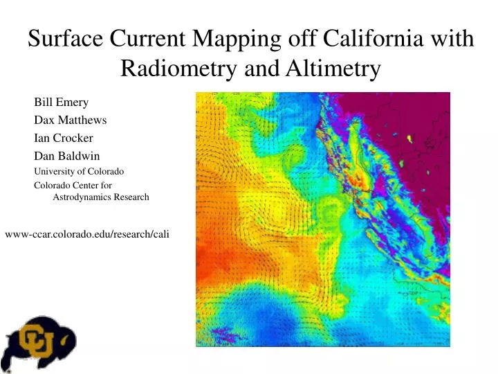
Surface Current Mapping off California with Radiometry and Altimetry. Bill Emery Dax Matthews Ian Crocker Dan Baldwin University of Colorado Colorado Center for Astrodynamics Research. www-ccar.colorado.edu/research/cali. Goals.

E N D
Surface Current Mapping off California with Radiometry and Altimetry Bill Emery Dax Matthews Ian Crocker Dan Baldwin University of Colorado Colorado Center for Astrodynamics Research www-ccar.colorado.edu/research/cali
Goals • 6-8 AVHRR BT images per day (requires automation), evaluate passive microwave SST and ocean color imagery for similar current calculations • Near Realtime system to produce updates of the mesoscale surface circulation in the California Current Region • Merge BT with altimeter data from Topex, Jason, ERS-1 , and ERS-2 satellites using the Optimal Interpolation Technique • Characterize the variability in time and space of the region’s mesoscale coastal surface currents
Tools • Maximum Cross Correlation (MCC) • SST imagery from AVHRR and AMSR • Ocean color imagery from MODIS • Cloud Filters • Image Navigator (Georegestration) • Quality Filters • Composites • Optimal Interpolation
Patterns are identified using cross correlations depicted in the first and second template boxes Position of the template in the first image is fixed, correlations are computed as the template in the second image is moved to different positions within the dashed line The template position with the greatest cross correlation indicates the most likely displacement of the feature Maximum Cross Correlation
Choosing the Areas • Choose the “template window” in the first image to have enough points to give a 95% significant correlation. • Choose the size of the search window in the second image large enough to be able to represent the maximum velocity between the images. • Filter the vectors for significant (high) correlations and for spatial coherence using a next-neighbor filter • Overlap the resulting vector windows to produce a high resolution spatial velocity field from the 1 km resolution imagery.
Sampling Issues • Altimeters are accurate but space between even the tandem mission tracks are too large to adequately resolve the mesoscale • Satellite imagery provides a 1 km spatial sample that is unfortunately frequently obscured by clouds • Can we combine the best attributes of both altimetry and imagery to produce accurate, timely and well-resolved maps of coastal surface currents. • Can these methods be used to compute a historical climatology as well as realtime updates for various applications needing accurate and high-resolution maps of coastal surface currents (seach&rescue, oil spills, etc.
History of MCC Method • First proposed for sea ice motion and then SST by Emery et al in 1986 • Kelly and Strub demonstrated that MCC was as accurate as other methods and easier to use • Many alternative methods have been proposed but nothing any easier or more accurate has been found • We have worked to develop methods to completely automate the MCC method so that it can be used in a near-realtime mode to map coastal surface currents and merge them with satellite altimeter derived currents.
Requirement for Accurate Navigation • To be useful for the MCC calculation the infrared and color images must be geolocated as accurately as possible (to within 1 km). • It is relatively easy to correct for geometric distortions but it is also necessary to correct for satellite attitude variations and for timing errors. • The MCC method itself can be used to create an method to automatically correct the images. • Once the geometric corrections have been made the MCC method is used to perform the final corrections for satellite attitude and timing.
Some Lessons Learned Over the Years Don’t use SST computed from satellite imagery. The SST algorithm uses a difference between two channels that are very similar which has the effect of amplifying the noise leading to lower correlations Use instead image brightness temperature
Cloud Filtering • Clouds Characteristics – Bright, cool, and have short time scales (for an individual pixel and compared to the ocean) • Albedo Threshold - Flags pixels which are brighter than a predetermined albedo (channel 2) • Temperature Threshold – Flags pixels which are cooler than a predetermined representative temperature • Temporal Threshold • Calculate mean and standard deviation for every pixel over a series of 10 days • Pixel is considered cloudy if its temp is lower than some value that depends on the maximum of the time series, adjusted empirically for temporal variations given by the standard deviation
Ocean Surface Currents • Determined by tracking thermal patterns from images 3 to 13 hours apart (MCC) • Using a 22 km template applied at 11 km intervals • Velocity found by dividing the calculated displacement by the time between the 2 images (assuming non-divergent flow) • Filtered using a variable correlation cutoff and a (3,2) next neighbor filter
Composites • Valid MCC vectors often exist at the same location for several consecutive days during an extended period of clear skies • Problematic for OI because of the size of the matrix computations required • Justified by noting that mesoscale currents are strongly auto-correlated over a few days time scale and hence daily MCC vectors are not strictly independent • Reduce MCC vectors by taking 3-day, 22 km composites
Optimal Interpolation • Also called Objective Analysis, first introduced to oceanography by Bretherton (1976) • OI makes an estimate of a variable from a weighted linear combination of observations made at irregular locations • Weights are chosen so that the estimate has the minimum expected ensemble mean square error • Mapping to a streamfunction is justified because mesoscale circulation is strongly geostrophic and hence weakly divergent • Mapping to a non-divergent streamfunction serves to largely filter out ageostrophic components of flow in the direct observations of velocity
MCC vs. Altimetry • Altimetry reveals geostrophic flow only – MCC data are interpreted as a total velocity that may include ageostrophic processes that advect thermal patterns • Even though thermal images are plagued by clouds, it has been shown that in certain regions the volume of MCC data can rival that of a satellite altimeter (Bowen et al. 2001) • MCC intermittently achieves higher resolution than altimetry • MCC has more observations near the coast, where the thermal gradients are pronounced, complementing altimeter data sampling
Problems with Merging • Even in some 3-day fields there will be very few MCC vectors and the OI merged vector velocities will depend primarily on the altimeter data as seen in this next example.
Example of Poor MCC Coverage • Here is a 3-day period with very few MCC vectors.
OI of Poor MCC w/Alt • This is the OI of the MCC vectors merged with altimetry for the same 3-day period.
OI Error of Poor Merged Field • You can see the large mapping errors except along the altimeter tracks as would be expected for no contribution from the MCC velocities.
Good 3-Day MCC Composite • This is a 3-day period of good MCC coverage particularly in the southeastern part of the region.
OI of Good MCC w/Alt • This is the OI of the MCC vectors merged with altimetry for the same 3-day period.
Error of Merged OI • This is the OI of the MCC vectors merged with altimetry for the same 3-day period. Note the improvement in the area covered by the MCC vectors.
Adding Ocean Color Imagery to Greatly Increase the Number of Images Available for MCC Surface Current Computations
Ocean Color Currents • This is an optimum interpolation of the 10-day composite of infrared and ocean color surface currents. The background is ocean color.
Ocean Color Currents 5 • This is an optimum interpolation of the 10-day composite of infrared and ocean color surface currents. The background image is infrared sea surface temperature
Comparing Altimetry with Ocean Color and Thermal Infrared Derived Surface Currents
Altimetry Optimum Interpolation (OI)September 13-16 2003 OI (red) of geostrophic surface currents from TOPEX/Poseidon and Jason
Altimetry and Ocean ColorSeptember 13-16 2003 OI Filtered Vectors
Altimetry and AVHRRSeptember 13-16 2003 OI Filtered Vectors
Exploring the Use of AMSR 6.7 GHz Imagery for Current Mapping
AMSR (6.7 GHz) Passive Microwave (red) with AVHRR (BW) July 6 - 16, 2003
AMSR (6.7 GHz) Passive Microwave (red) with AVHRR (BW) July 16 - 26, 2003
Advantage of Geostationary Orbit for MCC Current Mapping Frequent repeat coverage to find cloud free areas Problem: Lower spatial resolution Solution: Super resolution (the GAINS proposal)
First an example of super-resolution applied to AVHRR imagery over time. Uses the fact that with a precessing orbit the AVHRR never samples exactly the same spot; thus each location is oversampled over time.
The same area reconstructed from 20 images over 6 weeks yielding a resolution of 180 m….compare with Landsat, MSS
GEOSTATIONARY ADVANCED IMAGER FOR NEW SCIENCE GAINS Mission Statement Using a breakthrough technology called super-resolution to provide 1-km thermal infrared images from geosynchronous orbit, GAINS will monitor sea and land surface temperature in unprecedented detail to improve our understanding of the air-sea/land heat exchange. GAINS will enable numerous applications that require monitoring of thermal phenomena with high resolution in space and time. Science Objectives Resolve the diurnal cycle of sea and land surface temperature to 0.1 ˚C Detect and monitor wildfires with sufficient resolution to allow early prediction of the fires that will become dangerously destructive Compute ocean surface currents hourly and apply to Coast Guard search and rescue operations Mission Description Launched on 9/30/2005, GAINS will be placed into GTO and then use its own propulsion to enter GEO over the U.S.24 months of science operations, plus three more months to finish analysis
GAINS Instrument Developed by Raytheon Santa Barbara Remote Sensing, with significant heritage from existingsensors, including JAMI and MODIS Super-resolution technology achieves 1-km resolution with same aperture as current GOES sensor which has4-km resolutionSix channels — 3.7, 4.1, 8.6, 10.8, 12.0 µm, with an additional 3.7 µm low-gain channel for hot fires Spacecraft Ball BCP-2000 bus is a mature platform used on current and upcoming missions (QuikSCAT, ICESat, CloudSat) and is already being adapted for use in GEO Launch mass (with instrument and propellant) is 1352 kg
Conclusions: A GOES imager could provide the rapid repeat imagery needed to effectively find cloud-free image segments needed for MCC surface current mapping. 2. Super-resolution makes it possible to have a useful spatial resolution at GEO without a huge telescope