Download
1 / 51
540 likes | 707 Views
NRM Lec08. The reservoir: mechanistic model. Andrea Castelletti. Politecnico di Milano. Penstocks and turbine hall. Itaipu dam on the Parana river. Dam. Spillways in action. Three Gorges dam (China). Typical Localization. Clan canyon dam Colorado river. Longitudinal section.

E N D
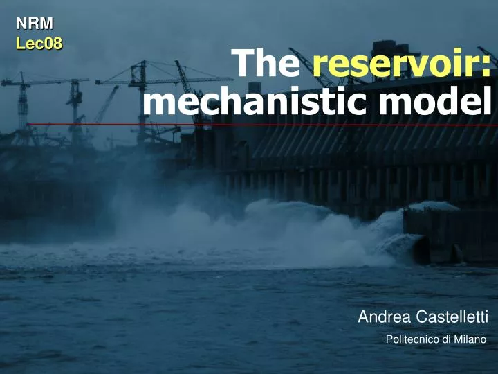
NRM Lec08 The reservoir:mechanistic model Andrea Castelletti Politecnico di Milano
Penstocks and turbine hall Itaipu dam on the Parana river Dam Spillways in action
Typical Localization Clan canyon dam Colorado river
Longitudinal section intake tower surface spillway intakes maximum storage bottom outlet water surface level minimum intake level penstock storage barrier
Bottom outlet Loch Lagghan dam Scozia
penstock • surface spillway
Gates: a) rising sector b) vertical rising c) radial Dam-gate structures
Piave - S.Croce system Reservoir network Hydropower reservoirs are often interconnected to form a network
Features of reservoirs By the management point of view a reservoir is characterized by: • the active (or live) storage; • the global stage-discharge curve of the spillways; • the stage-discharge curve of the intake tower;
Causal network st = storage volume at timet at+1 = inflow volume in [t ,t+1) rt+1 = effective release volume in [t , t+1)
Causal network What is missed? - evaporation - r depends ona and e
surface Mechanistic model What is missed? - evaporation - r depends ona and e
surface evaporation Mechanistic model
surface evaporation storage Mechanistic model
surface evaporation storage level Mechanistic model
surface evaporation storage level release Mechanistic model
balance net inflow balance net inflow estimator Cons Using it when the storage is not actually a cylinder generates an error. Balance equation Simplification: the storage is a cylinderS(st) = S Pros
Implicit assumption: the water surface is always horizzontal. arbitary constant Storage-level relationship There exist a biunivocal relationship between the level measured in a point and the storage. By inverting h(.) one obtains the value of the storage by measuring the level, i.e. the only measurable quantity Example:if the storage is a cylinder A negative storage represents the missing volume required to bring the water surface up to the level corresponding to the zero storage.
Implicit assumption: the water surface is always horizzontal. historic time series Storage-level relationship There exist a biunivocal relationship between the level measured in a point and the storage. By inverting h(.) one obtains the value of the storage by measuring the level, i.e. the only measurable quantity Non-cylindrical storage The identification of h(.) can be performed in different ways, depending on which one of the following is known: numerical computation point by point batimetry of the reservoir (DEM) interpolation
Examples of storage-level relationships Relazione invaso-quota Campotosto
Examples of storage-level relationships Relazione invaso-quota Piaganini
Examples of storage-level relationships Ricalibrazione scala
Surface-storage relationship Can be determined with similar techniques.
Continuous-time model of reservoir s(t) = storage volume at time t [m3] a(t) = inflow rate at time t [m3/s] i(t,s(t)) = infiltration [m3/s] e(t) = evaporation per surface area unit at time t [m/s] S(s(t)) = surface area [m2] r(t,s(t),p(t)) = release when the dam gate are open of p [m3/s]
Simplifications n(t) It depends on the storage-discharge functions and the position p of the intake sluice gates • i = 0almost always true, at least in artificial reservoirs • Cylindric reservoir n(t) = a(t)-e(t)S net inflow
Instantaneous storage-discharge relationships maximum release open gates minimum release limited spillway smin smax s* s(t) • s* :storage at wich spillways are activated • smin , smax:bounds of the regulation range
Example of storage-discharge relationship ~ N max (•) flow rate [m3/s] ~ N min (•) storage [Mm3]
Modelling for managing • The continuos-time model can not be used for managing: • decision are taken in discrete time instants • data are not always collected continuously discretize
st +nt+1 -rt+1 st = storage volume at time t nt+1 = net inflow volume in [t ,t+1) rt+1 = volume actually released in [t , t+1) t t +1 Discrete model of a reservoir st+1 = st +nt+1 -rt+1 nt+1= net inflow volume in [t , t+1) we assume it uniformly distributed nt+1
release decision with with 45° The release function rt+1 = Rt (st,nt+1 ,ut) Minimum dischargeable volume in [t , t+1) Maximum dischargeable volume in [t , t+1) givenst, &nt+1 givenst & ut rt+1 rt+1 Vt ut vt nt+1 ut
n = 50 m3/s n = 0 m3/s An example of minimum and maximum release (Campotosto, Italy) flow rate [m3/s] storage [Mm3]
depends on the inflow! Set of feasible controls U(st) feasible controlU(st) flow rate [m3/s] NO storage [Mm3]
45° Set of feasible controls U(st) stgiven rt+1 Vt (st,max{nt+1}) Vt (st,min{nt+1}) vt(st,max{nt+1}) vt(st,min{nt+1}) ut U(st)
releases of interest Remarks • vt(st ,nt+1)rt+1 Vt(st,nt+1) constraint already included inRt(•) NO • vt(st,nt+1)ut Vt(st,nt+1) • Ifnt+1is known rt+1 = ut • Alternative ways of formulating the mass balance equation ht =level at timet rt+1 = Rt(st ,nt+1 ,ut) = Rt (ht ,nt+1 ,ut) actual release in [t , t +1) nt+1= net inflow in terms of level rt+1= actual release in terms of level
CONCLUSIONS Model of a reservoir in operation state transition outputs feasible controls
CONCLUSIONS Model of a reservoir to be constructed
r a(s - smin)b 0 if ssmin N(s) = s smin Natural lake e h r a s hmin net or effective inflow Stage-discharge function N(s(t))
Linearization and time constant r a smin s D Linear continuos system tt+1 Lagrange formula a(s - smin) Remark:s(t+1) depends ons(t) only ifD<< T = a-1. T is the so-called time constant of the reservor.
Linearization and time constant r a smin s D Meaning of T tt+1 a(s - smin) By assumingD=T=1/aone gets Remark:s(t+1) depends ons(t) only ifD<< T = a-1. T is the so-called time constant of the reservor. T is the time required for the storage to reach 1/3 of its initial value.
Linearization and time constant r a smin s D tt+1 a(s - smin) Remark:s(t+1) depends ons(t) only ifD<< T = a-1. T is the so-called time constant of the reservor. An accurate modelling does require D<<T. Shannon’s or Sampling theorem
Time constant and the Lombardy lakes For most of the lakes T is nearly 8 days. LAKEST= a-1 [km2] [daysi] Maggiore 212.0 7.4 Lugano 48.9 8.7 Varese 15.0 34.7 Alserio 1.5 8.0 Pusiano 5.2 15.0 Como 146.0 7.7 Iseo 61.0 7.8 Garda 370.0 86.6 For ll these lakes the catchment areas is relatively small compared to the lake surface. The outlet mouth has not yet reached an equilibrium condition. The modelling time-step for lakes with T = 78 is about 1 day.
Buffering effecti.e. low-pass filtering dB 1/T w Bode diagram • Incoming waves whose frequency is smaller than 1/T are not smoothed. • E.g.: flood waves from snow melt. • Waves with frequency greater than 1/T are smoothed. • E.g.: flood waves from storms.
a a The modelling time-step depends upon the state To be sure that the system is well represented by the model: D 0,1*T Non-linear model: T is not defined Linearization of the system T changes with the values around which the system is linearized D changes with s It would be useful to have models with a time-step D that changes with s, however this is not possible with the algorithms nowadays available. Solution: use models with different D at different time steps.
Comparison between two lakes a2 >a1 r a2 a1 h h hmax t Average level
n Comparison between two lakes:impulsive flood P n* Average level t Impulse response Lake shore inhabitants Downstream users h r t t CONFLICT happy with lake 2 ( T small) Happy with lake 1 ( T big )
Lake regulation Lake shore population a big Downstream users a small Which compromise ? Natural lake Regulated lake r Natural regime curve Natural curve Curves for different gate positions h Different stage-discharge functions in different time instants
Lake regulation at r Downstream users at bt Lake popul. bt h(t) Months