Download
1 / 10
100 likes | 167 Views
The Simon Optimal Phase II Design (1989).

E N D
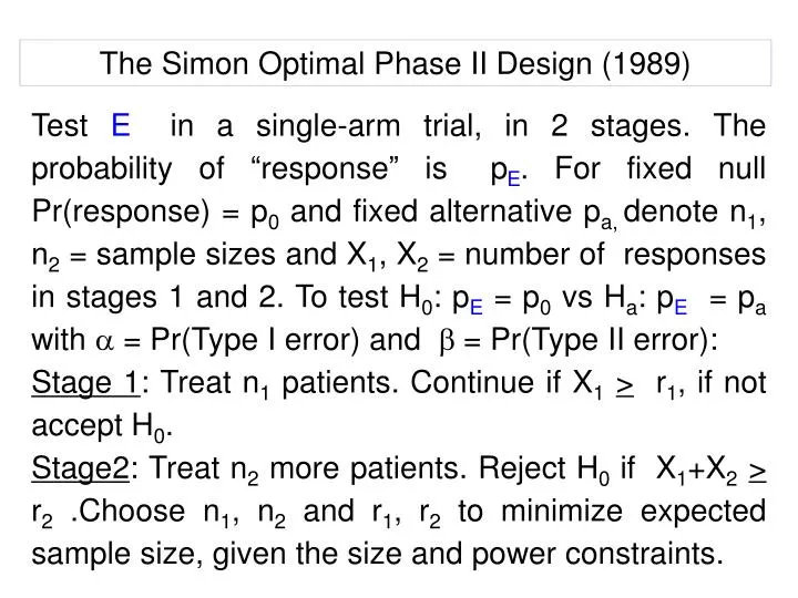
The Simon Optimal Phase II Design (1989) Test E in a single-arm trial, in 2 stages. The probability of “response” is pE. For fixed null Pr(response) = p0 and fixed alternative pa, denote n1, n2 = sample sizes and X1, X2 = number of responses in stages 1 and 2. To test H0: pE = p0 vs Ha: pE = pa with a = Pr(Type I error) and b = Pr(Type II error): Stage 1: Treat n1 patients. Continue if X1 > r1, if not accept H0. Stage2: Treat n2 more patients. Reject H0 if X1+X2 > r2 .Choose n1, n2and r1, r2to minimize expected sample size, given the size and power constraints.
Misinterpreting the Simon Design (Rattain, 2007) Suppose the null response probability with “standard” treatment is p0= .05. You wish to control a = .05 and b = .10 in phase II. Design 1: Target pa = .20 reject p0 =.05 if you observe > 5/41 (12.2%) responses Design 2: Target pa = .25 reject p0 =.05 if you observe > 4/30 (13.3%) responses Design 3: Target pa = .30 reject p0 =.05 if you observe > 3/17 (17.6%) responses For all 3 designs, the minimal empirical response rate to reject is < .20. What’s going on? One can only conclude p > .05, not p = pa . The “target” pa is artificial.
Some Simple Bayesian Analyses Assuming a beta(½,½) prior: 5/41 (12.2%) responses Pr(p >.20 | data)= .10, 95% ci [.048 - .247] includes p0= .05 and pa = .20. 4/30 (13.3%) responses Pr(p >.25 | data)= .062, 95% ci [.047 - .287] includes p0= .05 and pa = .25 3/17 (17.6%) responses Pr(p >.30 | data)= .131, 95% ci [.052 - .400] includes pa = .30, but also .25, .20, .25 and .10. None of these results are convincing evidence that p > pa. Is E really “promising”?
Frequentist Tests Reject p = .05 for target .20 Reject p = .05 for target .25 Reject p = .05 for target .30
An Ethical Problem With the Stopping Rule To test pa = .40 for experimental “E” vs p0= .20 with “standard” treatment, with a = .05 and b = .10 Stop interimly if < 4/19 responses, and reject p0 =.20 if you observe > 16/54 responses. But what if E is worse than the standard? When is it ethical to treat all n1 = 19 patients?
A Simple Solution Assume a Bayesian model, prior p~beta(.40, .60), (optimistic but uninformative), and monitor more frequently, at n=5, 10, 15, 19, stopping if Pr( p > .40 | data ) < .01 Pr(p > .40 | 0/5) = .0139 Continue Pr(p > .40 | 0/6) = .0077 STOP Pr(p > .40 | 1/10) = .0155 Continue Pr(p > .40 | 1/11) = .006 STOP
Ignoring Patient Heterogeneity in Phase II : An Example with Two Subgroups What if p0(Good)= .45 and p0(Poor)= .25 ? If Pr(Good) = Pr(Poor) = ½, the average null value is p0 = ½ .45 + ½ .25 = .35. A Simon design with a = .05 and b = .10 to test p0 = .35 versus pa = . 50 continues to stage 2 if there are > 20/53 responses. But what if E gives pa(Good)= .60 but pa(Poor)= p0(Poor)= .25 (treatment-subgroup interaction)?
2nd Example: A Typical Simon Phase II Design Test E in a single-arm trial using a Simon design comparing pE = p0 = .40 (response rate with standard therapy) to pE = pa = .60 with Pr(Type I error) = Pr(Type II error) = .10 Stage 1: Continue if > 8/18 responses Stage2: Conclude pE>.60 if >23/46 responses Go to phase III to compare Eto S
Bias From Phase II “Go - No GO” Rules If E has true pE = Pr(Response)=.40 (no improvement) and the design says E is“promising” if X18> 8 in stage 1 and X46> 23 in stage 2 then the final sample proportion X46 / 46 does not have mean .40 It has mean .527
Distribution of X46 / 46 after phase IIif true p = .40 Mean of X46 / 46 = .527 Mean = 0.527 The sample response rate X46 / 46 is on average MUCH larger than .40 simply due to the usual phase II “Go - No GO” rule to declare E “promising”