Download
1 / 39
390 likes | 487 Views
Application Layer Multicast. Overlay Networks. Treat the Internet as a physical network Build you own network on top of it In theory: all-to-all connectivity Challenge: make it efficient. Example: IP Multicast.

E N D
Overlay Networks • Treat the Internet as a physical network • Build you own network on top of it • In theory: all-to-all connectivity • Challenge: make it efficient
Example: IP Multicast • Multicast is an efficient delivery mechanism for Group-Communication applications. • IP Multicast • Relay on network layer to replicate and deliver data packets to receivers. • Problems with IP Multicast • Scales poorly with number of groups • Supporting higher level functionality is difficult • Deployment is difficult and slow
Application-Layer Multicast An alternative: provide multicast functionality above the IP layer i.e., Application-Layer or Overlay Multicast. • End-Hosts perform packet duplication and routing. • End-Hosts construct overlay network on unicast infrastructure
Efficiency of Multicast Trees • Challenge: construct efficient overlay trees • Application centric performance metrics: delay, throughput • Todays focus: delay optimized multicast trees • Naive Solution, Shortest Path Tree (SPT) • Does not limit node load • Creates bottlenecks (BW and CPU limits)
Efficiency of Multicast Trees (cont.) • Suggestions for Application-Layer multicast • Mesh First - Narada [CRZ00] • Tree First – Yoid [F99] • Minimal diameter trees [ST02],[BKKBS03] • Common Properties • Build ‘minimal’ diameter (height) trees with degree constrains • Low diameter Low delay • Low degree Low stress and bandwidth utilization
H1 H1 H1 Low-speed Link H3 H2 H2 R1 R2 H3 H3 H2 High-speed Links Efficiency of Multicast Trees (cont.) • Disadvantages: • Arbitrary selection of degrees • Requires trial and error • Ignores serialized message distribution • Scalability problem (known problem [CRZ00]) Non-Optimal Tree Optimal Tree
Todays Talk • New overlay network model • Map the node load to delay penalty • Quantifies multicast performance using a single delay metric. • Novelapproximation and heuristic algorithms • Generate delay optimized trees that intrinsically balance short latency with small degree • Suitable for delay-sensitive applications (audio-confreencing, CDN, etc) • Provides scalable solution • Performance analysis of structured overlay topologies
Processing Delay Communication Delay Sender host is free to handle other operations Message arrival Message Initiation The Overlay Network Model • A complete directed graph G=(V,E) • Communication cost function c : E R+ • Processing cost function p : V R+ • Sequential communication, p(v) is the minimum time interval between consecutive message transmissions of host v
The Minimal Delay Multicast (MDM)Problem Given a directed complete graph G=(V,E); a multicast group M V; a source host sM; a processing cost p(v), vV; and a communication cost c(e), eE; Finda scheme that minimizes the delay required to disseminate a message from s to all the other hosts in M. Only the hosts in M are allowed to participate in the distribution We assume that M≡V Group size n = |V|
The Ordered Tree Solution • Optimal solution is represented by an ordered tree T which spans V, rooted at s. • The i-th outgoing edge of node u corresponds to the i-th transmission from host u S 1 Notations Reception delay of v, tT(v) Tree cost, maxvV{tT(v)} 2 1 V1 V2 3 3 1 2 3 3 4 4 8 9 11 7 By Def. tT(s) =0 V3 V4 V5 V6
Optimal Multicast • Given a multicast tree T=(V,E) we calculate the optimal ordering using a recursive computation, working bottom-up. • Idea: The i-th delivery goes to the i-th largest cost subtree
Optimal Multicast – cont. • We neglect the ordering and concentrate on finding optimal tree • Optimal solution is a ‘non-lazy’ multicast scheme. S 10 1 2 1 V1 V2 8 5 2 1 3 3 4 4 0 0 0 0 V3 V4 V5 V6 • The optimal multicast problem is NP-Complete • Reduction from the telephone broadcast problem
Telephone Broadcast (TB) Problem • TB assumes a synchronous communication graph • In each communication round a node may send a message to at most one other node. • The problem is to notify the entire graph in minimal number of rounds. • Studied extensively, known to be NP-Complete [GJ79] • Reduction from TB problem • construct an overlay configuration with unit processing costs; zero communication costs for all the edges in E, and cost n for the rest.
Computation Models • Homogenous models • Active Networks [RS01] • Multicasting algorithm for line topologies • The heterogeneous postal model [BGNSS01] • Assumes undirected and complete graph G=(V,E) • Communication latency function λ • Switching (sending) time function s
Postal Approximation • log k approximation, k = size of multicast group • Inappropriate for overlay networks • Incorporates the sending time at the communication latency, whereas the overlay model incorporates this quantity at the processing delay. • sv λu,v, v,uV; Restricted cost model • Delay of the I-th message from u to v: • su*(i-1)+λu,vPostal Model • p(u)*i + c(u,v) Overlay Model • Doesn't support asymmetric costs
Our Approximation Approach Devise an approximation algorithm based on the postal approximation scheme • Define unrestricted cost model Generalized Heterogeneous Postal Model (GHP) • Adapt the postal approximation to support the GHP model. New approximation ratio: • Use a cost preserving transformation and invoke the adapted GHP approximation.
Postal Approximation Overview • Multicast problem: Find minimum time delivery from source r to a group of terminals U V. All the nodes in V may participate in the multicast. • Basic Idea • OPT ≥ 0.5 (LT*+∆T*) • T* - optimal multicast tree, spans U • LT* - maximum distance from r to any node in U • ∆T* - maximum generalized degree, the generalized degree of vU is its degree in T* multiplied by sv. • OPT - cost of the optimal solution • Find a multicast tree T which minimizes the quantity LT+∆T • NP-Complete problem
Postal Approximation • Iterative computation of the tree • At the i-th round use the Core proc. to compute • A core subset Ui Ui-1of size at most 0.75|Ui-1|, rUi • A dissemination schemefrom Ui to Ui-1, s.t the obtained time is linear in the optimal multicast time from r to Ui-1 • log |U| rounds log |U| approximation factor
Core(U’) Procedure • Find a set of |U’| paths, one for each terminal, where the path length and congestion (the generalized degree induced by the paths) is linear in LT*+∆T* • Use a multicommodity flow linear program to find a set of fractional paths that minimize the sum of two quantities: • L - the average length of the paths • ∆ - the congestion of the paths • The program ensures that L+ ∆ LT*+∆T* • Each flow path has length at most 4L • The total congestion is at most 6∆ • Round the set of fractional paths into integral paths
Core(U’) Procedure-Cont. • Transform the set of paths into a set of spider graphs • Each spider contains two nodes from U’ • The spiders span at least half of the nodes in U’ • The diameter and generalized degree of each spider is linear in LT*+∆T* • Include in the core an arbitrary node vU’ from each spider and all the nodes not contained in any spider.
GHP Adaptation • GHP support requires modification to the rounding mechanism only • Rounding Theorem [KLRTVV87] • Given a real matrix A, real vectors b,y, s.t Ay=b, a real value t ≥0 s.t in every column of A • The sum of all positive entries t • The sum of all negative entries ≥ -t Then, we can compute an integer vector y, s.t for every i
GHP Rounding matrix • Notations: • {Pi} is the set of fractional flow paths • E(Pi) and V(Pi) is the set of edges and nodes in Pi • f(Pi) is the amount of flow pushed on path I • Pjis the set of all paths from {Pi} which carry the j-th commodity • We use the following matrix for rounding the fractional paths:
GHP Rounding matrix-Cont. • The sum of the positive entries is at most 4Lα’ • The sum of the negative entries is at most -4Lα’ • Applying the rounding theorem, we get a set of integer paths s.t the length of each path 4Lα’, and the congestion 4Lα’+6∆ • Therefore, the length and the congestion are linear in (LT*+∆T*) α’
MDM Approximation Algorithm Input G=(V,E)edge costs c(u,v), node costs p(u), v,uV source host rV Algorithm Approx-MDM • Construct a GHP configuration (G,s,λ) s.t sv=p(v), vV; λu,v=0.5(p(u)+p(v))+c(u,v), eE; • Invoke the GHP approximation, assuming multicast group V, and source rV. • Return the computed tree
p3+p2 p1+p3 p1+p2 + + =λ3 =λ2 λ1 = + 2 2 2 c3 An Example =s1 p1 c1 c2 p2 =s2 s3= p3 c3 Path cost =c1+c3 +p3+ 0.5p1+0.5p2
Approximation Ratio Theorem 1: The approximation ratio of Approx-MDM is (OPT+pmax-pmin) O(log n) Cost of optimal tree Maximal processing cost Minimal processing cost Corollary: The approximation ratio for an overlay network with homogenous processing costs p(v)=p, vV OPT • O(log n)
Approximation ratio-Cont. GHP Notations • tGHPT(v) - reception delay of v • OPTGHP-cost of optimal solution Proof: • tGHPT(v) = tT(v)+ 0.5(p(v)-p(s)) , for any T, vV • OPTGHP OPT+ 0.5(pmax- pmin) • α 2 (α is the switching to communication ratio) The approximation ratio of the GHP approximation is at most OPTGHP •α •log n The theorem follows.
Heuristic Algorithm Approx-MDM suffers from high polynomial running time of Θ(n7). An alternative: a greedy algorithm Algorithm Heuristic-MDM Init: Add s to an empty tree 1. Compute the minimal reception delay of each non-notified host 2. Select the non-notified host with maximal reception delay 3. Add this host and the minimal latency path to the constructed tree Repeat 1-3 till all hosts are notified
Heuristic Algorithm - Cont. • Minimal latency path is computed using All-Pairs Shortest-Path (Floyd-Warshall) with weight matrix W=(wvi,vj) defined as: • Time complexity Θ(n3) • Supports arbitrary directed graphs
Homogenous Cost Overlays • Homogenous overlay network p(v)=p, vV; c(e)=c, eE • Any ‘non-lazy’ algorithm provides optimal solutions (e.g., Heuristic algorithm) Notations N(t), maximal number of hosts reached in time t. Rτ(t), maximal number of messages received in the interval (t-τ,t]
Convergence Rate inHomogenous Overlay Networks Lemma 3: Given an homogenous cost overlay Proof • There is one-to-one correspondence between the number of messages received in the interval (t,t+p] and the number of hosts which initiated processing in the interval (t-c-p,t-c] • Two types of hosts in the interval (t-c-p,t-c] • X, newly notified hosts • Y, hosts notified before t-c-p • Rp(t+p)= |X|+|Y|=|X|+N(t-c-p)=N(t-c)
Convergence Rate inHomogenous Overlay Networks Theorem 3: Given an homogenous cost overlay Corollary Any ‘Non-Lazy’ algorithm achieves logarithmic multicast delay, with the following bounds:
Simulation Results • The multicast delay for a clique topology with random costs from [1,10] • Max. latency is the weight of the longest path in the SPT • Problem is NP-Hard Use Max. latency as lower bound
Clique Topologies – Cont. • The multicast delay for a clique topology with random communication costs from [1,10] and unit processing costs • SPT has almost linear growth rate for large sizes
Power-Law Topologies • The multicast delay assuming random costs from [1,10] • Simulation based on power-law graphs (Notre-Dame Model [AB00]), average degree is 4.38.
Some Conclusions • Approximation Algorithm • High Computation Θ(n7) • Limited to small groups • Logarithmic height trees • Performance degradation in networks with dominating communication costs. • Support only complete undirected graphs • SPT • Suitable for small scale groups with dominating communication costs
Simulations Summary • On average the heuristic algorithm has a similar or better performance than the approximation algorithm • Heuristic trees are scalable for large group sizes • Near optimal result • Logarithmic like growth rate
Remarks • We can reduce the approximation ratio of the Approx-MDM algorithm to a pure logarithmic factor • Graphs in which the triangle equality holds may have better bounds