Download
1 / 65
730 likes | 1.02k Views
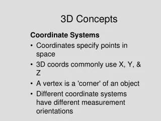
3D concepts and object representation . UNIT - 4. Introduction :. Up to here we have seen that how lines, circle, ellipse, characters etc can be drawn.

E N D
Introduction : Up to here we have seen that how lines, circle, ellipse, characters etc can be drawn. • In this unit, we will study the polygon representation methods – these methods are quite important because it’s the polygon that constitutes every closed object like tree, clouds, ball, car, etc., to be represented through graphics. • Further, each polygon has its own mathematical equation which works as the generating function for that polygon.
It’s the Bezier curves which have revolutionized the field of computer graphics and opened a new arena, i.e., automobile sector, for analysis and designing of automobiles. • Inspired with this achievement, scientists have worked hard and now there is no area which is complete without computer graphics and animation. In this unit, we will deal with fitting curves to the digitized data. • Two techniques are available for obtaining such curves cubic spline and parabolicaly blended curves.
1.1 3D display methods, • Polygon and quadric surfaces provide precise description for simple Euclidean objects like polyhedrons, ellipsoids. • Spline surfaces and construction techniques are useful for designing aircraft wings, gears, and other engineering structures with curved surfaces • Procedural methods such as fractals constructions and particle systems give us accurate representations for the natural objects like clouds, trees etc. • Physically based modeling methods using systems for interacting forces can be used to describe the non-rigid behaviors of piece of jelly, or a piece of cloth. • Octrees encoding are used to represent internal features of the objects, such as those obtained from medical CT images, volume renderings and other visualization techniques.
The representational schemes of solid objects are divided into two broad categories: • Boundary representations: Here the 3D object is represented as a set of surfaces that separate the object interior from the environment. Examples are polygonal facets and spline patches. For better understanding consider Figure 1. Figure 1
Space partitioning representations: These are used to describe the interior properties, by partitioning the spatial regions containing an object into a set of small non-overlapping contiguous solids (usually cubes). • Example: Octree (which is the space partitioning description of 3D object). For a better understanding consider Figure 2.
1.1.1 Polygon Surfaces • From Figure 1 and Figure 2 it is quite clear that it is possible to store object’s description as a set of surface polygons and the same is actually done by many graphic systems, actually this way of object description fastens the rendering and display of object surfaces. • The approach is beneficial because all the surfaces can now be described with linear equations and hence polygonal description of the surfaces is referred as “standard graphic objects”.
Consider Figure 3 where the cylindrical surface is represented as a mesh of polygons. The representation is known as wire frame representation which can quickly describe the surface structure. • On the basis of the structure a realistic rendering can be performed by interpolating the shading patterns across the polygon surfaces. • Thus polygon mesh representation of the curved surface is actually dividing a curved surface into polygon facets. • This improves and simplifies the process of rendering (transforming a 3D scene to 2D scene with least loss of information like height, depth etc).
Now the objects are composed of standard graphic objects (polygon surfaces). • Each graphic object needs some method for its description which could be a polygon table or equation etc.
1.1.2 Polygon Tables • Every polygon is analogous to a graph G(V,E). • So we can say that a polygon surface can be specified with as a set of vertex coordinates and associated attribute parameters (the attributes may be color, contrast, shading, etc). • Most systems use tables to store the information entered for each polygon, and it’s the data in these tables which is then used for subsequent processing, display and manipulation of the objects in the scene.
Polygon data tables can be organized into two groups: • Attribute tables: This table holds object information like transparency, surface reflexivity, texture characteristics, etc., of an object in the scene. • • Geometric tables: This table stores the information of vertex coordinates and parameters like slope for each edge, etc. To identify the spatial orientation of polygon surface. • In order to store geometric information of a polygon properly, this table is further bifurcated into three more tables:
In order to store geometric information of a polygon properly, this table is further bifurcated into three more tables: a) Vertex table: Holds coordinate values of vertices in the object. b) Edge table: Holds pointers back in to the vertex table for identification of the vertices related to each polygon edge. c) Polygon table or polygon surface table: Holds pointers back into the edge table for identification of the edges related to the polygon surface under construction.
Some basic tests that should be performed before producing a polygon surface by any graphic package: 1) every vertex is listed as an endpoint for at least two edges, 2) every edge is part of at least one polygon, 3) every polygon is closed, 4) each polygon has at least one shared edge, 5) if the edge table contains pointer to polygons, every edge referenced by a polygon pointer to polygon, every edge referenced by a polygon pointer has a reciprocal pointer back to polygon.
V1 E3 E6 E1 V3 V5 V2 E2 E4 E5 V4 Polygon Tables • Vertex Table • Edge Table • Surface Table
1.1.3 Plane Equation • Plane is a polygonal surface, which bisects its environment into two halves. One is referred to as forward and the other as backward half of any plane. Now the question is, which half is forward and which backward, because both are relative terms. • So we consider any point on the plane should satisfy the equation of a plane to be zero, i.e., Ax + By + Cz + D=0. • This equation means any point (x,y,z) will only lie on the plane if it satisfies the equation to be zero any point (x,y,z) will lie on the front of the plane if it satisfies the equation to be greater than zero, and any point (x,y,z) will lie on the back of the plane if it satisfies the equation to be less than zero.
Plane Equations • Ax+By+Cz+D=0 where x,y,z is any point on a plane • Three noncollinear points can determine A,B,C,D • Select (x1,y1,z1),(x2,y2,z2),(x3,y3,z3)
Plane Equations A=y1(z2-z3)+y2(z3-z1)+y3(z1-z2) B=z1(x2-x3)+z2(x3-x1)+z3(x1-x2) C=x1(y2-y3)+x2(y3-y1)+x3(y1-y2) D= -x1(y2z3-y3z2)-x2(y3z1-y1z3)-x3(y1z2-y2z1) • As vertex values and other information are entered into the polygon data structure, values for A, B,C and D are computed for each polygon and then can be stored with other polygon data.
1.1.4 Polygon Meshes • Construct the object from triangles or quadrilaterals by tiling • Most models are constructed this way • Easy to work with • Easy to render • Rates about 300 million triangles/sec available with ordinary graphics cards for PC computers
Polygon Meshes -triangular meshes- • Free form/Boolean disadvantages: complexity of description &algorithms • Representing a model as closed triangular mesh is EASY –Operations& Description format very simple • Base representation for scanned data • Most popular web representation
1.2 BEZIER CURVES AND SURFACES • It is the better technique to generate complex natural scenes is to use fractals. Fractals are geometry methods which use procedures and not mathematical equations to model objects like mountains, waves in sea, etc. • There are various kinds of fractals like self-similar, self-affined, etc. • Bezier curves, which is a Spline approximation method developed by the French engineer Pierre Bezier for use in the design of Renault automobile bodies.
Spline is a flexible strip used to produce a smooth curve through a designated set of points known as Control points ( it is the style of fitting of the curve between these two points which gives rise to Interpolation and Approximation Splines). • In computer graphics, the term spline curve now refers to any composite curve formed with polynomial sections satisfying specified continuity conditions (Parametric continuity and Geometric continuity conditions) at the boundary of the pieces, without fulfilling these conditions no two curves can be joined smoothly.
1.2.1 Bezier Curves • Bezier curves are used in computer graphics to produce curves which appear reasonably smooth at all scales. • The Bezier curve require only two end points and other points that control the endpoint tangent vector. • Bezier curve is defined by a sequence of N + 1 control points, P0, P1,. . . , Pn. • We defined the Bezier curve using the algorithm (invented by DeCasteljeau), based on recursive splitting of the intervals joining the consecutive control points.
De Casteljeau algorithm: The control points P0, P1, P2 and P3are joined with line segments called ‘control polygon’, even though they are not really a polygon but rather a polygonal curve. • Each of them is then divided in the same ratio t : 1- t, giving rise to the another points. Again, each consecutive two are joined with line segments, which are subdivided and so on, until only one point is left. This is the location of our moving point at time t. The trajectory of that point for times between 0 and 1 is the Bezier curve.
A simple method for constructing a smooth curve that followed a control polygon p with m-1 vertices for small value of m, the Bezier techniques work well. However, as m grows large (m>20) Bezier curves exhibit some undesirable properties.
Bezier curves are commonly found in painting and drawing packages, as well as CAD system, since they are easy to implement and they are reasonably powerful in curve design.
Spline Development • First-order splines find straight-line equations between each pair of points that • Go through the points • Second-order splines find quadratic equations between each pair of points that • Go through the points • Match first derivatives at the interior points • Third-order splines find cubic equations between each pair of points that • Go through the points • Match first and second derivatives at the interior pointsNote that the results of cubic spline interpolation are different from the results of an interpolating cubic.
Cubic Splines • While data of a particular size presents many options for the order of spline functions, cubic splines are preferred because they provide the simplest representation that exhibits the desired appearance of smoothness. • Linear splines have discontinuous first derivatives • Quadratic splines have discontinuous second derivatives and require setting the second derivative at some point to a pre-determined value. • Quadratic or higher-order splines tend to exhibit the instabilities inherent in higher order polynomials (ill-conditioning or oscillations)
Cubic Splines (cont) • In general, the ith spline function for a cubic spline can be written as: • For n data points, there are n-1 intervals and thus 4(n-1) unknowns to evaluate to solve all the spline function coefficients.
Given a set of control points, cubic interpolation splines are obtained by fitting the input points with a piecewise cubic polynomial curve that passes through every control points. • Suppose we have n+1 control points with coordinates : • Pk=(xk,yk,zk) where k = 0 to n
We can describe the parametric cubic polynomial that is to be fitted between each pair of control points with the following set of equations : - • x(u) = axu3 + bxu2 + cxu + dx • y(u) = ayu3 + byu2 + cyu + dy • z(u) = azu3 + bzu2 + czu + dz
Hermite Form • Let’s look at an alternative way to describe a cubic curve • Instead of defining it with the 4 control points as a Bezier curve, we will define it with a position and a tangent (velocity) at both the start and end of the curve (p0, p1, v0, v1)
Hermite Curve v1 v0 • p1 • p0
Hermite Curves • We want the value of the curve at t=0 to be x(0)=p0, and at t=1, we want x(1)=p1 • We want the derivative of the curve at t=0 to be v0, and v1 at t=1
Hermite Curves • The Hermite curve is another geometric way of defining a cubic curve • We see that ultimately, it is another way of generating cubic coefficients • We can also see that we can convert a Bezier form to a Hermite form with the following relationship:
B-Spline • The degree of a Bezier Curve is determined by the number of control points • E. g. (bezier curve degree 11) – difficult to bend the "neck" toward the line segment P4P5. • Of course, we can add more control points. • BUT this will increase the degree of the curve increase computational burden
B-Spline • Joint many bezier curves of lower degree together (right figure) • BUT maintaining continuity in the derivatives of the desired order at the connection point is not easy or may be tedious and undesirable.
B-Spline – moving a control point affects the shape of the entire curve- (global modification property) – undesirable. • Thus, the solution is B-Spline – the degree of the curve is independent of the number of control points • E.g - right figure – a B-spline curve of degree 3 defined by 8 control points
B-Spline • In fact, there are five Bézier curve segments of degree 3 joining together to form the B-spline curve defined by the control points • little dots subdivide the B-spline curve into Bézier curve segments. • Subdividing the curve directly is difficult to do so, subdivide the domain of the curve by points called knots 0 u 1
B-Spline • In summary, to design a B-spline curve, we need a set of control points, a set of knots and a degree of curve.
Knots and Knot vectors of B-splines • Knot • Each subinterval endpoint ui • Knot Vector • Entire set of selected subinterval endpoints • Choose any values for subinterval endpoints • Only condition ui <=u i +1 • u min and u max depend on • The number of control points we select (n) • Value for d (degree)