Download
1 / 51
510 likes | 639 Views
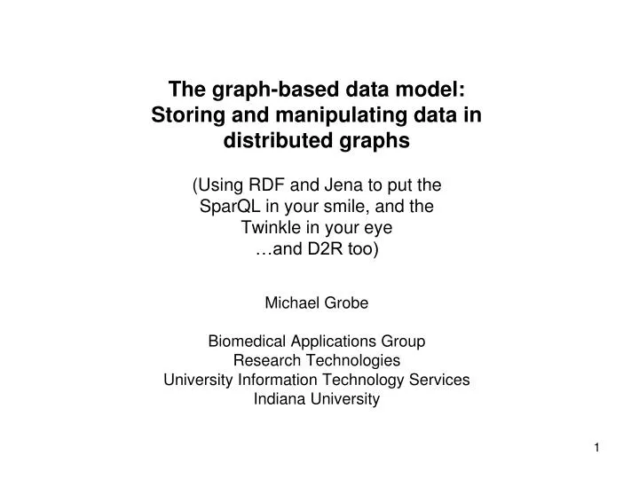
The graph-based data model: Storing and manipulating data in distributed graphs (Using RDF and Jena to put the SparQL in your smile, and the Twinkle in your eye …and D2R too) Michael Grobe Biomedical Applications Group Research Technologies University Information Technology Services

E N D
The graph-based data model: Storing and manipulating data in distributed graphs (Using RDF and Jena to put the SparQL in your smile, and the Twinkle in your eye …and D2R too) Michael Grobe Biomedical Applications Group Research Technologies University Information Technology Services Indiana University
This presentation in perspective This is actually one of a series of presentations on Linked Data Web and graph database technologies: Introduction to ontologies This presentation on RDF, Jena, SparQL, etc OWL and inference over ontologies Using graph technologies in bioinformatics research In general, these topics appear “simple”, but are fraught with complications, limitations, and qualifications…especially when the casual user attempts to compare them with relational data approaches to the same or similar problems. In addition, this is a pretty big elephant surrounded by a lot of “blind men”. As a result, this presentation is a survey of concrete examples of basic components used to manipulate data using stored as graphs, or “appearing to have been” stored in graphs. It will use the Gene Ontology for some of these examples.
Table of Contents Using graphs to represent data Using RDF to represent graphs Jena – a Java class library for manipulating RDF Using SparQL graph templates to query RDF Using Twinkle to make SparQL queries Using iSPARQL graphical graph templates to query RDF Exposing relational data as RDF Thinking of SparQL queries as SQL Table of Non-contents OWL and inference over ontologies Using the Semantic Web in bioinformatics research
Using graphs used to represent data Here are 2 graphs that represent 2 kinds of information associated with 4 different persons. Graph #1: Person ages Graph #2: Favorite Friends
Using graphs to represent data Here the 2 graphs are combined using named edges to represent 2 kinds of information associated with the same 4 persons. Graph #3: Person ages (:age) and favorite friends (:fav) Read these links as “Smith has age 21” or “Jones has favorite friend Smith” to make them more “sentence-like”. Each arc is like the “predicate” of a sentence, connecting a “subject” with an “object”. (Note that a subject may have >= 0 arcs of each type.)
Using graphs to represent data Data is sometimes represented using so-called “blank nodes” to help cluster attributes together. Graph #4: Blank nodes linking a name, an age, and a favorite friend via arcs named :name, :age, and :fav, as follows: Blank nodes are useful for specifying lists of items, but are discouraged within the Semantic Web. Use (dereferenceable) URIs (like “http://www.iu.edu/”) whenever possible.
Using URIs and URLs to represent data Now if it hadn’t already happened someone could come up with the idea to use URLs to point to Web documents that describe the “exact” meaning of each edge. For example, some popular magazine could publish their definition of “favorite friend” on a page like http://CelebrityMagazine.com/fav and other documents could define “BFF”, “long-time-friend”, “family-friend”, etc, And, in fact, these definitions could themselves refer to other definitions like some “superset” of relationships such as: http://SomeCelebrityMagazine.com/personal_relationships or the personal_relationships file, itself, could include a collection of definitions, including “favorite friend, or “fav”, that we might refer to as: http://SomeCelebrityMagazine.com/personal_relationships#fav using the # convention for targeting a specific location within a URL. Of course, for a lot of applications this would all be unnecessary; some URI could just be used to indicate an edge type known to the file creator.
Using RDF-XML to serialize graphs Graphs can be “serialized” or represented in a textual format. When graphs are serialized, each connection is represented by 3 components, a so-called RDF “triple”. Each triple is composed of a “subject”, “predicate” and “object” where each edge between each pair of entities becomes a named “predicate”. Each subject is represented as: - a blank node, such as “_2”, - a literal value, such as “value”^^type where type is some URI, that defines a data type, as in “21”^^:age, or - a URI, like http://fake.host.edu/smith Each object is represented as: - a blank node - a literal value, or - a URI Each predicate is represented as: - a URI, like http://fake.host.edu/contact-schema#fav, or an abbreviated URI like example:age which represents a URI that will be expanded by substituting a value for the string“example”. If the specified URI is dereferenceable to a URL, that URL may identify a text file that defines the meaning (or semantics) of the predicate. (Some writers speak of “object”, “property”, and “property value”.)
Graph #3 as a set of 12 triples (3 for each person) |-------------------------------------| | Subject | Predicate | Object | ======================================= | “Blake” | example:fav | “Blake” | | “Blake” | example:age | "12" | | “Blake” | example:name | "Blake" | | | “Jones” | example:fav | “Smith” | | “Jones” | example:age | "35" | | “Jones” | example:name | "Jones" | | | “George” | example:fav | “Smith” | | “George” | example:age | "21" | | “George” | example:name | "George" | | “Smith” | example:fav | “Jones” | | “Smith” | example:age | "21" | | “Smith” | example:name | "Smith" | --------------------------------------- Here the abbreviation “example:” stands for http://fake.host.edu/example-schema#
Two ways to represent the Graph #3 triples using RDF-XML Properties encoded as XML entities: <rdf:RDF xmlns:rdf="http://www.w3.org/1999/02/22-rdf-syntax-ns#" xmlns:example="http://fake.host.edu/example-schema#"> <example:Person> <example:name>Smith</example:name> <example:age>21</example:age> <example:fav>Jones</example> </example:Person> </rdf:RDF> Properties encoded as XML attributes: <rdf:RDF xmlns:rdf="http://www.w3.org/1999/02/22-rdf-syntax-ns#" xmlns:example="http://fake.host.edu/example-schema#"> <rdf:Description example:name=“Smith” example:age=“21” example:fav=“Jones” </rdf:Description> </rdf:RDF>
Representing URIs In work with RDF you will see URIs abbreviated in several ways, using: namespace, PREFIX and ENTITY definitions, depending on the context : xmlns:lib=“http://some.host.edu/directory” or PREFIX <lib:http://some.host.edu/directory> or !ENTITY lib “http://some.host.edu/directory” If the namespace abbreviations in the entities example above get “expanded”, then Smith is actually being represented as: <rdf:RDF xmlns:rdf="http://www.w3.org/1999/02/22-rdf-syntax-ns#" <http://fake.host.edu/example-schema#Person> <http://fake.host.edu/example-schema#name> Smith </http://fake.host.edu/example-schema#name> <http://fake.host.edu/example-schema#age> 21 </http://fake.host.edu/example-schema#age> <http://fake.host.edu/example-schema#fav Jones </http://fake.host.edu/example-schema#fav"> </http://fake.host.edu/example-schema#Person> </rdf:RDF>
Graph #3 using “resources” to represent each person Persons are modeled as “resources” by replacing the strings for each node identifier with URIs: ------------------------------------------------------------------------------- | Subject | Predicate | Object | =============================================================================== | <http://fake.host.edu/blake> | example:fav | <http://fake.host.edu/blake> | | <http://fake.host.edu/blake> | example:age | "12" | | <http://fake.host.edu/blake> | example:name | "Blake" | | | | <http://fake.host.edu/jones> | example:fav | <http://fake.host.edu/smith> | | <http://fake.host.edu/jones> | example:age | "35" | | <http://fake.host.edu/jones> | example:name | "Jones" | | | | <http://fake.host.edu/george> | example:fav | <http://fake.host.edu/smith> | | <http://fake.host.edu/george> | example:age | "21" | | <http://fake.host.edu/george> | example:name | "George" | | | | <http://fake.host.edu/smith> | example:fav | <http://fake.host.edu/jones> | | <http://fake.host.edu/smith> | example:age | "21" | | <http://fake.host.edu/smith> | example:name | "Smith" | ------------------------------------------------------------------------------- Here the abbreviation “example” stands for http://fake.host.edu/example-schema# These URIs need not be dereferenceable.
Representing entries in Graph #3 as “resources” Format 1 <rdf:RDF xmlns:rdf="http://www.w3.org/1999/02/22-rdf-syntax-ns#" xmlns:example="http://fake.host.edu/example-schema#"> <example:Person rdf:about=“http://fake.host.edu/smith”> <example:name>Smith</example:name> <example:age>21</example:age> <example:fav rdf:resource=“http://fake.host.edu/jones” /> </example:Person> </rdf:RDF> - - - - - - - - - - - - - - - - - - - - - - - - - - - - - - - - - - Format 2 <rdf:RDF xmlns:rdf="http://www.w3.org/1999/02/22-rdf-syntax-ns#" xmlns:example="http://fake.host.edu/example-schema#"> <rdf:Description about=“http://fake.host.edu/smith” example:name=“Smith” example:age=“21” /> <example:fav rdf:resource=“http://fake.host.edu/jones” /> </rdf:Description> </rdf:RDF> Note that the resource URI references in this example are not “real” documents; they are not “dereferenceable”.
A person record using FOAF (from Obitko) <rdf:RDF xmlns:rdf="http://www.w3.org/1999/02/22-rdf-syntax-ns#" xmlns:foaf="http://xmlns.com/foaf/0.1/" xmlns="http://www.example.org/~joe/contact.rdf#"> <foaf:Person rdf:about= "http://www.example.org/~joe/contact.rdf#joesmith"> <foaf:mbox rdf:resource="mailto:joe.smith@example.org"/> <foaf:homepage rdf:resource="http://www.example.org/~joe/"/> <foaf:family_name>Smith</foaf:family_name> <foaf:givenname>Joe</foaf:givenname> </foaf:Person> </rdf:RDF>
RDF summary and implications for the Semantic Web A graph may be represented as a collection of triples. RDF-XML representations of graphs will contain URIs that: - serve to identify and/or reference syntactic elements (they define tag names), and - identify and/or name “resources”: subjects, predicates and/or objects. Such URIs may be “imaginary” or provide addresses of actual, “dereferenceable”, web documents, in possibly remote locations. This can result in a “Gigantic Global Graph”, usually know as the Linked Data Web or the “Semantic Web,” with RDF as one of W3C’s Semantic Web architectural levels. “If HTML and the Web make all online documents look like one huge book, RDF, schema, and inference languages will make all the data in the world look like on huge database.” TimBL [Editor’s note: Here TimBL is using the term “schema” to refer to an RDF schema that defines RDF triples much more loosely than a relational database schema defines a collection of tables in a database.]
RDF graphs may be interrogated: - by physical inspection (for anyone willing to read XML) - by writing programs that read RDF files, construct the represented graphs internally, and then - access graph triples in sequential order, - select triples according to specified content, and/or - apply SparQL queries and access results in sequential order - using command-line tools that apply SparQL queries - using GUI interfaces accepting SparQL queries - written in text, or - represented graphically - via URLs carrying form data, or SOAP requests to SparQL endpoints
How to query an RDF graph using Jena The Java-based Jena package from HP Labs allows users to manipulate and query graphs, and import/export RDF, etc. You can write a program that uses Jena classes to - retrieve and parse an RDF file containing a graph or a collection of graphs, - store it in memory, and then - examine each triple in turn, examine one component (say, the subject) of each triple in turn, or examine only triples that meet specified criteria. For example, one might examine each stored triple searching for a specific reference URI, or for a specific literal value. One might look for persons of a specific age, “21”^^xsd:age, in the object portion of each triple. Jena also provides support for inference using rule sets and for querying via SparQL.
Jena example In JENA, RDF nodes can have type “Resource”, “URI Resource”, “literal”, or anonymous (slight extension to standard RDF). A Jena model is created by a factory: Model m = ModelFactory.createDefaultModel(); A Jena ontological model is a model along with a “reasoner”(sic): OntModel m = ModelFactory.createOntologyModel(); Jena can - read in an RDF serialized graph (from a file, URL, etc.) - write a serialized model to a file or STDOT, and - perform standard operations on the model. For example, given the populated models m and n, Jena can then do: Model x = m.add( n ); // Union Model y = m.remove( n ); // Set difference Model z = m.intersection( n ); // Set intersection - save and retrieve model data in/from a database
Reading and writing a model in Jena String input FIleName = “Some-GO-entries-diddled.rdf”; Model m = ModelFactory.createDefaultModel(); InputStream in = FileManager.get().open( inputFileName ); if( in == null ) { throw new IllegalArgumentException( “File not found.\n” ) } model.read( in, ““ ); // Treat blank lines as nulls. model.write( System.out [, {“N-triple”|”RDF/XML”|”XML-ABBREV”}] ); //which will yield a file of N-triple, RDF/XML, or XML-ABBREV records.
Cannonical process to examine each triple in a model stmtIterator iterator = model.listStatements(); // Statements composed of triples while( iterator.hasNext() ) { Statement statement = iterator.nextStatement(); Resource subject = statement.getSubject(); Property predicate = statement.getPredicate(); // Get the object, which in this example, may be a Resource or just a string, so // it is kept in an RDFNode, a superclass of Resource and literal. RDFNode object = statement.getObject(); // superclass of Resource and literal // Now process the object; here it is just printed. System.out.print( subject.toString() ); System.out.print( “ “ + predicate.toString() ); if( object instanceof Resource ) { // it’s a resource. System.out.print( “ “ + object.toString() ); } else { // it’s a literal that will be printed with surrounding quotes. System.out.print( “ \“” + object.toString() + “ \“” ); } }
Statement iterators for accessing selected components There are several methods for creating iterators over a model: - Some simply list the components of each triple: - model.listSubjects(); - model.listObjects(); - Some compare a specific component with a specified value, as in: model.listSubjectsWithProperty( Prop p, RDFNode o); (which will get you a collection of subjects possessing property/predicate p and specific value o) - Some compare all components against specific values in 2 steps: - define a “selector” possessing specific values s, p and o, where null or (RDFNode) null matches anything: Selector selector = new SimpleSelector( subject, predicate, object ) - and then build the statement list: model.listStatements( selector );
SparQL: a graph-based query language Sparql is a language that lets users query RDF graphs . . . using graph patterns (written in N3) containing variables. The query engine will return an exhaustive list of triples that satisfy each query through value substitution. (aka “query by example”, QBE). This process is not always intuitive, and/or “SQL has perverted the minds of a generation of programmers” (J. Random Guy somewhere on the Web). SparQL is implemented in Jena through the ARQ package, and queries may be made from within Java scripts (McCarthy, 2005), or via a SparQL client distributed with Jena. The process to make a query is: - build a query in a .rq file, and - execute the query using: sparql –query filename.rq or sparql.bat –query filename.rq SparQL does not do inference (except when used within Jena against an ontological model).
A SparQL example This SparQL example query simply asks for a list of the first 10 triples in the file specified in the FROM clause: PREFIX rdf: <http://www.w3.org/1999/02/22-rdf-syntax-ns#> PREFIX example: <http://fake.host.edu/example-schema#> select $s $o from <http://kongo.uits.iupui.edu:8546/rdf-example-1.rdf> where { $s $p $o . } LIMIT 10 $s, $p, and $o are variable names that will each be assigned a value as the query is “satisified.” Variable names may also start with “?”.
SparQL: a graph-based query language The basic, partial syntax of a SparQL query is based on N3(/turtle) and similar to: BASE <some URI from which relative FROM and PREFIX entries will be offset> PREFIX prefix_abbreviation: < some_URI > SELECT some_variable_list FROM <some_RDF_source > WHERE { { some_triple_pattern . } . } Notes: - the “<“ and “>” characters are required literals, - the BASE and PREFIX entries are optional and BASE applies to relative URIs appearing in either PREFIX or FROM clauses, - SELECT may be replaced by CONSTRUCT, ASK, or DESCRIBE, - * is a valid variable list, and may be preceded by DISTINCT - there may be multiple FROM clauses, which will be treated as a single store, - the term WHERE is optional, and may be omitted, and - while this syntax resembles SQL, it has very different semantics.
Querying Graph #3 format 1 using SparQL Here’s a reminder of one of the representations used to store of Graph #3 here stored in a file named rdf-example-1.rdf: <?xml version="1.0" encoding="UTF-8"?> <rdf:RDF xmlns:rdf="http://www.w3.org/1999/02/22-rdf-syntax-ns#" xmlns:example="http://fake.host.edu/example-schema#" > <example:Person rdf:about="http://fake.host.edu/smith"> <example:name>Smith</example:name> <example:age>21</example:age> <example:fav rdf:resource="http://fake.host.edu/jones" /> </example:Person> </rdf:RDF>
A SparQL query against the first data representation C:\Jena-2.5.7\Jena-2.5.7\bat> cat query-example-1.rq PREFIX rdf: <http://www.w3.org/1999/02/22-rdf-syntax-ns#> PREFIX example: <http://fake.host.edu/example-schema#> select * from <http://kongo.uits.iupui.edu:8546/smiht-format-1.rdf> where { $s $p $o . } C:\Jena-2.5.7\Jena-2.5.7\bat> sparql.bat --query query-example-1.rq ------------------------------------------------------------------------------ | s | p | o | ============================================================================== | <http://fake.host.edu/smith> | example:fav | <http://fake.host.edu/jones> | | <http://fake.host.edu/smith> | example:age | "21" | | <http://fake.host.edu/smith> | example:name | "Smith" | | <http://fake.host.edu/smith> | rdf:type | example:Person | ------------------------------------------------------------------------------- (Were you expecting a graph? CONSTRUCT will produce one.)
Querying Graph #3 format 2 using Sparql Here’s a reminder of the other representation of Graph #3 stored in a file named rdf-example-2.rdf: <?xml version="1.0" encoding="UTF-8"?> <rdf:RDF xmlns:rdf="http://www.w3.org/1999/02/22-rdf-syntax-ns#" xmlns:example="http://fake.host.edu/example-schema#" > <example:Person rdf:about="http://fake.host.edu/smith" example:name=“Smith” example:age=“21” /> <example:fav rdf:resource="http://fake.host.edu/jones" /> </example:Person> </rdf:RDF>
The same SparQL query against the second data representation C:\Jena-2.5.7\Jena-2.5.7\bat> cat query-example-2.rq PREFIX rdf: <http://www.w3.org/1999/02/22-rdf-syntax-ns#> PREFIX example: <http://fake.host.edu/example-schema#> select * from <http://kongo.uits.iupui.edu:8546/smith-format-2.rdf> where { $s $p $o . } C:\Jena-2.5.7\Jena-2.5.7\bat> sparql.bat --query query-example-2.rq ------------------------------------------------------------------------------ | s | p | o | ============================================================================== | <http://fake.host.edu/smith> | example:fav | <http://fake.host.edu/jones> | | <http://fake.host.edu/smith> | example:age | "21" | | <http://fake.host.edu/smith> | example:name | "Smith" | ------------------------------------------------------------------------------
A “distributed” SparQL query against 4 separate RDF files The next query searches 4 dereferenceable files holding “live” data in the first representation format above: C:\Jena-2.5.7\Jena-2.5.7\bat> cat query-example-all.rq PREFIX rdf: <http://www.w3.org/1999/02/22-rdf-syntax-ns#> PREFIX example: <http://fake.host.edu/example-schema#> select * from <http://kongo.uits.iupui.edu:8546/smith> from <http://kongo.uits.iupui.edu:8546/jones> from <http://kongo.uits.iupui.edu:8546/george> from <http://kongo.uits.iupui.edu:8546/blake> where { $s $p $o . } If the data were all in one file, only one FROM clause would have been required.
Results of the distributed SparQL query C:\Jena-2.5.7\Jena-2.5.7\bat> sparql.bat --query query-example-all.rq ------------------------------------------------------------------------------------------- | s | p | o | ============================================================================================ | <http://kongo.uits.iupui.edu/blake> | example:fav | <http://kongo.uits.iupui.edu/blake>| | <http://kongo.uits.iupui.edu/blake> | example:age | "12" | | <http://kongo.uits.iupui.edu/blake> | example:name | "Blake" | | <http://kongo.uits.iupui.edu/blake> | rdf:type | example:Person | | <http://kongo.uits.iupui.edu/jones> | example:fav | <http://kongo.uits.iupui.edu/smith>| | <http://kongo.uits.iupui.edu/jones> | example:age | "35" | | <http://kongo.uits.iupui.edu/jones> | example:name | "Jones" | | <http://kongo.uits.iupui.edu/jones> | rdf:type | example:Person | | <http://kongo.uits.iupui.edu/george> | example:fav | <http://kongo.uits.iupui.edu/smith>| | <http://kongo.uits.iupui.edu/george> | example:age | "21" | | <http://kongo.uits.iupui.edu/george> | example:name | "George" | | <http://kongo.uits.iupui.edu/george> | rdf:type | example:Person | | <http://kongo.uits.iupui.edu/smith> | example:fav | <http://kongo.uits.iupui.edu/jones>| | <http://kongo.uits.iupui.edu/smith> | example:age | "21" | | <http://kongo.uits.iupui.edu/smith> | example:name | "Smith" | | <http://kongo.uits.iupui.edu/smith> | rdf:type | example:Person | -------------------------------------------------------------------------------------------- In this query all 4 files were searched as if they were in a single file. Note that the URI contents are different in this live example.
The magic of “ontologies” There are many defintions of “ontology”, but in very general terms, an “ontology” may be thought of as a “taxonomy” of objects (or concepts) based on a particular relationship between pairs of those objects (or concepts). A common example of a taxonomy is an “evolutionary tree” in which individual species are related on the basis of evolutionary descent. That is, one species of each pair connected by an edge descended from the other. (Actually, it’s the members of the species who evolve, but . . .) Within such structures no member is considered to have descended from more than one immediate species. Within an ontology,” however, an object or concept may have more than one immediate “parent,” and no circular sub-graphs are allowed, so the resulting structure is a Directed Acyclic Graph (DAG). An ontology can be represented by a “special” RDF graph: It is special in that the predicates convey transitivity: if A is a descendant of B, and B is a descendant of C, then A is a descendant of C. IS_A and PART_OF relationships are commonly used to build ontologies.
Here is a portion of the GO is_a DAG (Ashburner, 2004) for molecularfunction (example: “chromatin binding” is_a “DNA binding”) (Note that this diagram shows some genes, but the Gene Ontology is actually a taxonomy of terms that can be used to describe or annotate genes, rather than a taxonomy of genes. )
Here’s the first entry (of the ~26K) in the GO text version (with all three parts intermixed) [Term] id: GO:0000001 name: mitochondrion inheritance namespace: biological_process def: "The distribution of mitochondria, including the mitochondrial genome, into daughter cells after mitosis or meiosis, mediated by interactions between mitochondria and the cytoskeleton." [GOC:mcc, PMID:10873824, PMID:11389764] synonym: "mitochondrial inheritance" EXACT [] is_a: GO:0048308 ! organelle inheritance is_a: GO:0048311 ! mitochondrion distribution You can also get the GO as RDF XML, or as a MySQL database. A portion of the molecular function extract on the previous page is shown in RDF XML on next page:
<?xml version="1.0" encoding="UTF-8"?> <rdf:RDF xmlns:rdf="http://www.w3.org/1999/02/22-rdf-syntax-ns#" xmlns:go="http://www.geneontology.org/dtds/go.dtd#"> <go:term rdf:about="http://www.geneontology.org/go#all"> (Note: “all” is like “root”.) <go:accession>all</go:accession> <go:name>all</go:name> <go:definition>This term is the most general term possible</go:definition> </go:term> <go:term rdf:about="http://www.geneontology.org/go#GO:0003674"> <go:accession>GO:0003674</go:accession> <go:name>molecular_function</go:name> <go:synonym>GO:0005554</go:synonym> <go:synonym>molecular function</go:synonym> <go:definition>Elemental activities, such as catalysis or binding, describing the actions of a gene product at the molecular level. A given gene product may exhibit one or more molecular functions.</go:definition> <go:is_a rdf:resource="http://www.geneontology.org/go#all" /> </go:term> </rdf:RDF> <go:term rdf:about="http://www.geneontology.org/go#GO:0005488"> <go:accession>GO:0005488</go:accession> <go:name>binding</go:name> <go:synonym>ligand</go:synonym> <go:definition>The selective, often stoichiometric, interaction of a molecule with one or more specific sites on another molecule.</go:definition> <go:is_a rdf:resource="http://www.geneontology.org/go#GO:0003674" /> </go:term>
Find parents of GO:0004003 in the example GO subset PREFIX xsd: <http://www.w3.org/2001/XMLSchema#> PREFIX rdf: <http://www.w3.org/1999/02/22-rdf-syntax-ns#> PREFIX go: <http://www.geneontology.org/dtds/go.dtd#> select * from <http://discern.uits.iu.edu:8421/Some-GO-entries- diddled.rdf> where { <http://www.geneontology.org/go#GO:0004003> go:is_a $parent . } Result: C:\Jena-2.5.7\bat> sparql.bat --query GO-paths-from-4003.rq ----------------------------------------------- | parent | =============================================== | <http://www.geneontology.org/go#GO:0008094> | | <http://www.geneontology.org/go#GO:0008026> | | <http://www.geneontology.org/go#GO:0003678> | ----------------------------------------------- (This query takes about 30 seconds on the whole GO RDF-XML file, using the java parameters -Xss4m -Xms30m -Xmx1500m)
Find all 3-element paths up from GO:0004003 PREFIX go: <http://www.geneontology.org/dtds/go.dtd#> select * from <http://discern.uits.iu.edu:8421/Some-GO-entries-diddled.rdf> where { <http://www.geneontology.org/go#GO:0004003> go:is_a $a . $a go:is_a $b . $b go:is_a $c . } Note that given a table showing the GO DAG, you can get this result within SQL using multiple joins, but you can’t find N-element paths in either language (unless you use inference within SparQL).
Find all 3-element paths up from GO:0004003 using Twinkle (A similar query found that 19 GO classes have the maximum hop count of 15 to the GO root.)
Query dbpedia for entries about “Goethe” (using Virtuoso iSparql text query) Note that the predicate “bif:contains” is a Virtuoso “Built-In Function” that searches back-end text indexes. It might be possible to search using a standard SparQL regex FILTER, but it would be much slower.
The same query using the iSparql “graphical” QBE interface Here is the same query in graphical form as constructed using the iSparql QBE interface: Components can be dragged-and-dropped from the menu at the top of the window. The whole interactive window is shown on the next page.
Possible applications for ontologies Suppose uniprot.org provides a list of 89K proteins, their mappings to NCBI Gene IDs, and their GO annotations (which it does), and perhaps a small subset looks like: XXX GO:00003682 YYY GO:00003682 ZZZ GO:00008026 AAA GO:00008096 And suppose go.org links GO IDs with GO category names, which it does, And suppose I have a list of researchers and their various areas of interest, like Smith studies gene XXX Jones studies nucleic acid binding etc. Then . . . what kinds of questions can I ask that would have been difficult before, like: What research interests do Smith and Jones have in common? Who might be interested in collaborating on DNA helicase activity?
Optional clauses in SparQL queries SparQL has more features than presented so far. Here are some clauses permitted following the “where” clause: order by [DESC|ASC| ] ( variable_list ) limit n: print up to n return values. offset n: start output with the nth return value. 43
Optional clauses in SparQL queries Permitted within “where” clauses: FILTER: restricts variable matches in the preceding triple to specified filter patterns, as in: { $s $p $date FILTER ( $date > "2005-01-01T00:00:00Z"^^xsd:dateTime ) } or { $s $p $d FILTER ( xsd:dateTime( $d ) < xsd:dateTime( "2005-01-01T00:00:00Z“ ) ) } or { ?s ?p ?name FILTER regex( ?name, "^smi", “some_flag“ ) } UNION: “where” clauses may be constructed as { triple_pattern_1 } UNION { triple_pattern_2 } and any RDF element matching either of these triples will be included in the resulting output. OPTIONAL { triple_pattern }: identifies a triple that need not appear in an RDF target but whose absence will not prohibit a pattern match. GRAPH: directs a query to apply a triple to a specified RDF source, possibly defined by a variable: GRAPH some_RDF_source { another_triple_pattern . } . or GRAPH some_variable { yet_another_triple_pattern . } .
“A relational view of the Semantic Web” (Newman, 2007) Relaxing certain requirements normally imposed upon SQL (specifically type contraints on joined fields), there are strong similarities among operations applied to relational and graph-based models. For example: - triple_pattern . triple_pattern approximates an “untyped” join, as demonstrated on the next slide - filter approximates an SQL conditional - union approximates an outer union - optional approximates a left outer join( R, S ), which join( R, S ) unioned with an anti-join( R, S), where an anti-join difference with a semi-join, and a semi-join join and a projection.
“A relational view of the Semantic Web” (Newman, 2007) Here we look at the triple pattern used to find the 3 hop paths towards the GO root node, select $a, $b, $c where { <http://www.geneontology.org/go#GO:0004003> go:is_a $a . $a go:is_a $b . $b go:is_a $c . } Which is roughly equivalent to the following SQL query: select a.parent_id, b.parent_id, c.parent_id from GO.molecular_function_DAG a join GO.molecular_function_DAG b on a.parent_id = b.child_id join GO.molecular_function_DAG c on b.parent_id = c.child_id where a.child_id like 'GO:0004003'
Publishing relational data as “virtual” RDF stores So far we have accessed RDF presented mostly from free-standing files. However, legacy relational databases can be published as RDF stores on the Semantic Web by using gateways like D2R and Virtuoso (commercial). The D2R approach requires 2 steps: - interrogate the database via JDBC using generate-mapping to build a configuration (mapping) file from the relational table definitions, and then - start the D2R server with the mapping file. Notes: - Each table row becomes a separate resource/graph. - Primary keys (if any) become resource identifiers, and - rows in linked tables identified by foreign keys may be merged into the entity (?). The D2R utility dump-rdf can also convert an entire table into RDF form for access in a single SparQL query.
Accessing data via a “SparQL Endpoint” Since the D2R server makes a “SparQL endpoint” available, one can execute queries via HTTP requests like http://kongo.uits.iupui.edu:6700/sparql?query= select ?s ?p ?o where{ ?s ?p ?o .} limit 10 The D2R server also provides a Web form that can be used to interrogate its content using SparQL. This interface is based on an AJAX component called SNORQL, and available at http://kongo.uits.iupui.edu:6700/sparql The D2R server also provides an interface for users to browse its backend data. To use it you just “Web in” to: http://kongo.uits.iupui.edu:6700
Portion of a D2R-server mapping file for CLSD @prefix map: <file:/C:/d2r-server-0.4/mapping-clsd2-GO-DGN.n3#> . @prefix d2rq: <http://www.wiwiss.fu-berlin.de/suhl/bizer/D2RQ/0.1#> . map:database a d2rq:Database; d2rq:jdbcDriver "com.ibm.db2.jcc.DB2Driver"; d2rq:jdbcDSN "jdbc:db2://libra45.uits.iu.edu:50000/clsd2"; d2rq:username “account"; d2rq:password “password"; . # Table DISEASE_GENE_NET.GENES map:DISEASE_GENE_NET_GENES a d2rq:ClassMap; d2rq:dataStorage map:database; d2rq:uriPattern "DISEASE_GENE_NET.GENES/@@DISEASE_GENE_NET.GENES.GENE_ID@@"; d2rq:class vocab:DISEASE_GENE_NET_GENES; . map:DISEASE_GENE_NET_GENES__label a d2rq:PropertyBridge; d2rq:belongsToClassMap map:DISEASE_GENE_NET_GENES; d2rq:property rdfs:label; d2rq:pattern "DISEASE_GENE_NET.GENES #@@DISEASE_GENE_NET.GENES.GENE_ID@@"; . For each field in the table there is an entry like: map:GENES_GENE_ID a d2rq:PropertyBridge; d2rq:belongsToClassMap map:DISEASE_GENE_NET_GENES; d2rq:property vocab:GENES_GENE_ID; d2rq:column "DISEASE_GENE_NET.GENES.GENE_ID"; d2rq:datatype xsd:long; .
Triple stores There exist so-called “triple stores” that can use backend data storage engines, like MySQL, to house RDF data, and process queries. For example, Sesame is a triple store that can use serveral different kinds of backends: DBMS (originally PostgreSQL), simple RDF files, and/or other, network-accessed triple stores, like Sesame itself. Sesame also demonstrates a “generic architecture” for RDF and RDFS storage and query processing, and does not require keeping the whole graph in memory, when processing requests. Jena can also employ back-end data base management systems. There are also some graph based data management systems, like Neo4j, that can be used to store raw graph structured data. In fact, Neo4j has at least one overlay product that uses Neo4j to manage RDF. Neo4j may work well for data collections running into the billions of nodes, since it does not require its whole graph to be memory-contained (although it works better with larger memory), and is quite fast. .