Download
1 / 45
450 likes | 635 Views
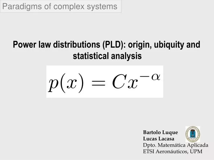
Paradigms of complex systems. Power law distributions (PLD): origin, ubiquity and statistical analysis. Bartolo Luque Lucas Lacasa Dpto. Matemática Aplicada ETSI Aeronáuticos, UPM. Critical phenomena Phase transitions Edge of chaos Domain of power laws. Index.

E N D
Paradigms of complex systems Power law distributions (PLD): origin, ubiquity and statistical analysis Bartolo Luque Lucas Lacasa Dpto. Matemática Aplicada ETSI Aeronáuticos, UPM
Critical phenomena • Phase transitions • Edge of chaos Domain of power laws
Index • Introduction to PLD: typical scale range. • Mechanisms by which PLD can arise. • Other broad dynamic range distributions. • Detecting and describing PLD: tricky task. Appendix: stable laws
Introduction 1.1What is a power law distribution (PLD) ? 1.2 Where do we find PLD’s ?
Typical scale Many of the things that scientists measure have a typical size or scale. For instance, the heights of human beings vary, but have a typical size between 50 cm and 272 cm, the ratio being around 4. The mean is around 180 cm. In complex networks : random graphs
In complex networks : scale free networks Not all the things we measure are peaked around a typical value, or have a typical size. Some vary over an enormous dynamic range. The distribution of city sizes Log-log plot The system shows an unexpected symmetry NO typical value or a typical scale (all sizes, all scales).
Distributions of that form are called Power Law Distributions (PLD), and have the following functional shape: where a is the so called exponent and C can be obtained by normalization. PLD with finite size effects Pure PLD
WHERE ? • statistical physics: critical phenomena, edge of chaos, fractals, SOC, scale-free networks,... • geophysics: sizes of earthquakes, hurricanes, volcanic eruptions... • astrophysics: solar flares, meteorite sizes, diameter of moon craters,... • sociology: city populations, language words, notes in musical performance, citations of scientific papers... • computer science: frequency of access to web pages, folder sizes, ... • economics: distributions of losses and incomes, wealth of richest people,... • a huge etc. • What (universal?) mechanisms give rise to this specific distribution? • How can we know with rigor when a phenomenon shows PLD behavior?
2. Mechanisms by which PLD can arise * 3.1 Combinations of exponentials. 3.2 Random walks (self-similar motion, fractals). * 3.3 The Yule process: rich gets richer * 3.4 Phase transitions and critical phenomena. * 3.5 Self-organized criticality (SOC). 3.6 Random multiplicative processes with constraints. 3.7 Maximization of generalized Tsallis Entropy (correlated /edge of chaos systems). Others: Coherent-noise mechanism, highly optimized tolerant (HOT) systems, etc
2.1 Combinations of exponentials. Exponential distribution is more common than PLD, for instance: • Survival times for decaying atomic nuclei • Boltzmann distribution of energies in statistical mechanics • etc... - Suppose some quantity y has an exponential distribution - Suppose that the quantity we are interested in is x, exponentially related to y Where a, b are constants. Then the probability distribution of x is a PLD
2.1 Combinations of exponentials: example – biologically motivated • Process where a set of items grow exponentially in time (population or organisms reproducing without constraints) . • In this process a death process takes place, the probability of an item to die increasing exponentially (in other words, the probability of still living decreases exponentially with time) . • Thus, the “still living items distribution” will follow a power law APPLICATIONS: - Sizes of biological data - Incomes - Cities - Population dynamics - etc
Also known as • The gibrat principle (Biometrics) • Matthew effect • Cumulative advantage (bibliometrics) • Preferential attachment (complex networks) 2.3 The Yule process (rich gets richer) • Initial population • With t, a new item is added to the population • how?? With probability p, to the most relevant one! with probability 1-p, randomly. Initial population Time (more nodes)
PLD’s 2.4 Critical phenomena: Phase transitions. Global magnetization 1. T=0 well ordered 2. 0<T<Tc ordered 3. T>Tc disordered
2.5 Critical phenomena : Self-organized criticality (SOC). 2.5 Self-organized criticality (SOC). SELF ORGANIZED CRITICALITY
Sandpile model : celular automata sandpile applet • A grain of sand is added at a randomly selected site: z(x,y) -> z(x,y)+1; 2. Sand column with a height z(x,y)>zc=3 becomes unstable and collapses by distributing one grain of sand to each of it's four neighbors. This in turn may cause some of them to become unstable and collapse (topple) at the next time step. Sand is lost from the pile at the boundaries. That is why any avalanche of topplings eventually dies out and sandpile "freezes" in a stable configuration with z(x,y)<=z everywhere. At this point it is time to add another grain of sand.
Los modelos SOC se pueden entender como primeras aproximaciones a modelos de turbulencia, donde la energía (avalanchas, arena) es disipada a todas las escalas, con correlaciones espaciales descritas por un exponente de Kolmogorov generalizado (exponente crítico). • Otras descripciones matemáticas de turbulencia: multifractales (también aparecen PLD’s).
Resumen: dos mecanismos fundamentales • Proceso de Yule: proceso evolutivo por el que se generan distribuciones espaciales de tipo ley de potencias. “Rich gets richer”. • Fenómenos críticos y SOC: escalas o tamaños típicos de un sistema divergen: - si acercamos el sistema a un punto crítico: transiciones de fase. - si el sistema evoluciona de forma natural a ese punto crítico: SOC.
3. Other broad dynamic range distributions * 3.1 Log-normal distributions: multiplicative process 3.2 Stretched exponential distributions. 3.3 PLD with exponential cutoff.
3.1 Log-normal distributions: multiplicative process • At every time step, a variable N is multiplied by a random variable. • If we represent this process in logarithmic space, we get a brownian motion, as long as log() can be redefined as a random variable. • log(N(t)) has a normal (time dependent) distribution (due to the Central Limit Theorem) • N(t) is thus a (time dependent) log-normal distribution. Now, a log-normal distribution looks like a PLD (the tail) when we look at a small portion on log scales (this is related to the fact that any quadratic curve looks straight if we view a sufficient small portion of it).
A log-normal distribution has a PL tail that gets wider the higher variance it has.
Example: wealth generation by investment. • A person invests money in the stock market • Getting a percentage return on his investsments that varies over time. • In each period of time, its investment is multiplied by some factor which fluctuates (random and uncorrelatedly) from one period to another. Distribution of wealth: log-normal
4. Detecting and describing PL: tricky task. 4.1 Logarithmic binning. 4.2 Cumulative distribution function. 4.3 Extracting the exponent: MLE vs. graphical methods. 4.4 Estimation of errors: goodness-of-fit tests.
4.1 Logarithmic binning • first insight: a histogram of a quantity with PLD appears a straight line when plotted on log scales. Noise (fluctuations) Generation of 106 random numbers drawn from a PLD with exponent 2.5 • noise is due to sample errors: there are too few data in many intervals, which give rise to fluctuations. • however, we can’t throw out the data in the tail, because many distributions follow PL in the tail we need to avoid those fluctuations.
4.1 Logarithmic binning • In order to avoid these tail fluctuations, we have to bin wider in the tail (in order to take into account more data in each bin): a way to make a varying binning (the most common) is the logarithmic binning. • note: we have to normalize each binning by its size, in order to get a count per unit interval. Less fluctuations. Some noise is still present. Why? # of samples falling in the kth bin decreases with the exponent of the PLD if this exponent is greater than one. Every PLD with exponent greater than 1 is expected to have noisy tails.
4.2 Cumulative distribution function • Another method of plotting the data (in order to avoid fluctuations): instead of plotting the histogram, we plot the cumulative distribution function: probability that x has a value greater or equal to X: It’s intuitive that fluctuations are absorbed, so that binning is no more a problem. If p(x) follows a PLD, P(x) too: But with a different exponent Histogram Logarithmic binning Cumulative
NOTATION • Distributions plots are called histograms. • Histograms that follow PLD are called power laws. • Cumulative distributions are called rank/frequency plots. • Rank/frequency plot which follow a PLD are called Zipf laws (if the plot is P(x) vs. x) or Pareto ditributions (if the plot is x vs. P(x)).
4.3 Exponent estimation of the PLD • The first attempt is to simply fit the slope of the straight line in the log-log plot (least squares, for instance). In our example, this leads to wrong results: Fitted . . . . . . Expected . . . slope
Why a simple fitting of the slope doesn’t usually work? Fitting to a PLD by using graphical methods based on linear fit on log-log is: • inaccurated • Biased : extreme data . Sometimes, the fitted exponent is not accurate, some others, the underlying process does not generate PLD data, and the shape is due to outside influences, such as biased data collection techniques or random bipartite structures. • Example Generation of 104 random numbers drawn from a PLD with exponent 2.5 (50 runs) Graphical methods
Maximum likelihood estimate of exponents (MLE) Given a PLD, applying normalization, we get Given a set of n values xi, the probability that those values where generated from a PLD with exponent a is proportional to the likelihood of the data set: and the probability that a is the correct exponent is related through Bayes theorem: Applying the usual MLE ( searching the extrema of ln( ) ) we find: Where xmin in practice is not the smallest value but the smallest one for which the PL behavior holds. Now, which is the goodness-of-fit of MLE ? =
4.4 Estimation of errors: Kolmogorov-Smirnov test (KS) KS test is based on the following test statistic: where is the hypothesized cumulative distribution function, is the empirical distribution function (based on sample data). Method:KS seeks to reject the PLD hypothesis • Estimate, using MLE, the power law exponent. • Look for the maximum distance between the hypothesized cumulative distribution and the empirical (cumulative) distribution. • Taking into account the # of samples, check the quantile Q. • The Observed Significance Level OSL = (1-Q)% • When OSL > 10%, there is insufficient evidence to reject the hypothesis that the distribution is PLD
4.4 Estimation of errors: Pearson’s c2 where: Oi = an observed frequency Ei= an expected (theoretical) frequency, asserted by the null hypothesis Now you compare your result with the specific table, in order to reject or not the null hypothesis (hyp: the observed data don’t come from the expected –theoretical- distribution).
APPENDIX_____________ Stable Laws and their relation to Power law distributions
Stable Laws: GAUSSIAN and LEVY LAWS Def Summing N i.i.d random variables with pdf P1, one obtains a random variable which Is in general a different pdf Pn given by N convolutions of P1. Distributions such that Pn has the same form that P1 are said to be stable. This property must hold, up to translations and dilations (affine transformations). Pn(x’)dx’ = P1(x)dx , where x’ = anx + bn Note A stable law correspond to a fixed point in a Renormalization Group process. Fixed Points of RG usually play a very special role: attractive fixed points (as this case) describe the macroscopic behavior observed in the large N limit. The introduction of correlations may lead to repulsive fixed points, which are the hallmark of a phase transition, i.e. the existence of a global change of regime at the macroscopic level under a variation of a control parameter quantifying the strength of the correlations.
Stable Laws: GAUSSIAN and LEVY LAWS Gaussian law The best-known example of a stable law is the Gaussian law, also called the normal law or the Laplace-Gauss law. For instance, the Binomial and Poisson distributions tend to the Gaussian law under the operation of addition of a large number of random variable (the central limit theorem is an explanation to this fact). where is the mean Gaussian law is the variance Log-Normal law A variable X is distributed according a log-normal pdf if lnX is distributed according a gaussian pdf. The log-normal distribution is stable, not under addition but under multiplication (i.e., addition in the log space) not stable in rigor! But interesting to talk about. This pdf can be mistaken with a PLD, over a relatively large interval (up to 3 decades, depending of the value of ). In fact, we can express this pdf as a PLD with exponent that goes like -1-ln(x)/2 (when is big, the exponent looks constant).
Stable Laws: GAUSSIAN and LEVY LAWS The Lévy laws Paul Lévy discovered that in addition to the Gaussian law, there exists a large number of stable pdf’s. One of their most interesting properties is their asymptotic Power law behavior. Asymptotically, a symmetric Lévy law stands for P(x) ~ C / |x|1+for x infinity • C is called the tail or scale parameter • is positive for the pdf to be normalizable, and we also have <2 because for higher values, the pdf would have finite variance, thus, according to the Central Limit theorem, it wouldn’t be stable (convergence to the gaussian law). At this point a generalized central limit theorem can be outlined. There are not simple analytic expressions of the symmetric Lévy stable laws, denoted by L (x), except for a few special cases: • =1 - Cauchy (Lorentz) law - L1(x) = 1/(x2 + p2) • = 1/2 with C=1
Stable Laws: GAUSSIAN and LEVY LAWS Lévy versus gaussian
Bibliography • Power laws, Pareto distributions and Zipf´s law, M.E.J. Newman • Critical phenomena in natural sciences, D. Sornette • Problems with Fitting to the PLD M. Goldstein, S. Morris, G.G. Yen • Logarithmic distributions in reliability analysis B.K. Jones • A Brief History of Generative Models for Power Law and Lognormal Distributions M. Mitzenmacher
Also known as • The gibrat principle (Biometrics) • Matthew effect • Cumulative advantage (bibliometrics) • Preferential attachment (complex networks) 2.3 The Yule process (rich gets richer) Suppose a system composed of a collection of objects (cities, papers, etc). What we wish to explain is why a certain property of these these collection of objects (number of citizens, number of citations, etc) is distributed following a very precise kind of distribution: PLD. The variable under study is k (number of citations of papers, size of cities, etc): the unity • New objects appear once in a while, as people publish new papers for instance. • Newly appearing objects have some initial k0. • In between the appearance of a new object (a new city, a new paper), m new people/citations/etc are added to the entire system, in proportion to the number of people/citation that the city/paper already has, for every object. (rich gets richer) • Note: to overcome the problem when k0=0, we can assign new citations not in proportion simply to k, but to k+c, where c is some constant. PARAMETERS OF THE MODEL: k0 , c , m Evolutive argument
Let pk,nbe the fraction of objects that have k unities when the total number of objects is n. Thus the number of such unities is npk,n. It can be shown that the master equation of this process is: With stationary solution , where and Now, the beta-function follows a power law distribution in its tail, with exponent a, thus we can conclude that the Yule process generates a power law distribution pk with exponent a related to the three parameters of the process.
Susceptible to small changes 2.5 Self-organized criticality (SOC). Certain extendeddissipative dynamical systems naturally evolve into a critical state, with no characteristic time or length scales. The temporal “fingerprint” of the welf-organized critical state is the present of 1/f noise, its spatial signature is the emergence of scale-free (fractal) structures. Per Bak et al., Phys. Rev. A 38 (1988) Example : Sandpile (BTW) cellular automata model • The system drives itself towards its attractor by generating avalanches of all sizes. Moreover, the attractor is the critical state!! (In phase transitions, the critical state is unstable). • As long as the system reaches the critical state, it will maintain there generating avalanches of all sizes (no characteristic length). (Distribution of avalanches follow PLD for instance). Applications: Geophysics, Economics, Ecology, Evolutionary biology, Cosmology, Quantum gravity, Astrophysics, Sociology, etc.
Starting with an arbitrary configuration and repeating the above procedure brings the system to a stationary state, where for every grain of sand added to the system on average precisely one grain of sand is lost at the boundary. • It is clear that the system in this state must have large avalanches. Indeed, addition of a grain of sand at one of the central sites would not cause the loss of sand (which is required by stationarity) unless the chain reaction of topplings isn't able to propagate all the way to the boundary, which is exactly the definition of large (system-wide) avalanche. • It turns out that in this delicately balanced steady state the distribution of avalanche sizes (measured as total number of topplings in the avalanche) follows a scale-free power law distribution: P(S) ~ S-1.2 . In other words, the system operates in a critical state (in the sense of equilibrium physics of second order phase transitions). Notice that this critical state is a unique attractor of the dynamical rules, conserving sand everywhere except for the boundaries. Hence the name Self-Organized Criticality.