Download
1 / 71
720 likes | 879 Views
COP 4600 – Summer 2012 Introduction To Operating Systems Uni-processor Scheduling. Instructor : Dr. Mark Llewellyn markl@cs.ucf.edu HEC 236, 407-823-2790 http://www.cs.ucf.edu/courses/cop4600/sum2012. Department of Electrical Engineering and Computer Science

E N D
COP 4600 – Summer 2012 Introduction To Operating Systems Uni-processor Scheduling Instructor : Dr. Mark Llewellyn markl@cs.ucf.edu HEC 236, 407-823-2790 http://www.cs.ucf.edu/courses/cop4600/sum2012 Department of Electrical Engineering and Computer Science Computer Science Division University of Central Florida
In a multiprogramming system, multiple processes exist concurrently in main memory. Each process alternates between using the processor and waiting for some event to occur, such as the completion of I/O. The key to multiprogramming is scheduling. The goals of scheduling are: Assign processes to be executed by the processor(s) Improve response time Improve throughput Increase processor efficiency Uni-processor Scheduling
There are typically four different types of scheduling involved. Long-term scheduling: The decision to add to the pool of processes to be executed. Medium-term scheduling: The decision to add to the number of processes that are partially or fully in main memory. Short-term scheduling (dispatcher): The decision as to which available process will be executed by the processor. I/O scheduling: The decision as to which process’s pending I/O request will be handled by an available I/O device. (We’ll defer this type of scheduling until we discuss I/O management later in the course.) Types of Scheduling
Levels of Scheduling This diagram reorganizes the state transition diagram to suggest the nesting of scheduling functions. Scheduling affects the performance of the system because it determines which processes will wait and which will progress. This is illustrated by the next diagram.
Determines which programs are admitted to the system for processing Long term scheduling controls the degree of multiprogramming The decision as to when to create a new process is general driven by the desired degree of multiprogramming. The more processes that are created, the smaller is the percentage of time each process can be executed (i.e., more processes are competing for the same amount of processor time). Thus, the long term scheduler may limit the degree of multiprogramming to provide satisfactory service to the current set of processes. Long-Term Scheduling
The decision as to which job to admit next can be based on a simple first-come-first-served basis, or it can be based on a much more elaborate protocol to assist in the management of system performance. Many different criteria can be used including: Priority Expected execution time I/O requirements Overall system balance (CPU bound versus I/O bound processes) Note: for time sharing systems, process creation will occur when a user attempts to connect to the system. Time sharing users are not queued up and kept waiting, rather all comers are accepted until the system reaches some saturation point. Long-Term Scheduling (cont.)
Part of the swapping function. Typically the swapping-in decision is based on the need to manage the degree of multiprogramming. On a system that does not use virtual memory, memory management also becomes an issue that must be addressed by the medium-term scheduler. This means that the swapping-in decision must consider the memory requirements of the swapped-out process. Medium-Term Scheduling
In terms of frequency of execution, the long-term scheduler executes relatively infrequently and makes the coarse-grained decision of whether or not to take on a new process and which one to take. The medium-term scheduler is executed somewhat more frequently to make a swapping decision. The short-term scheduler is also known as the dispatcher, executes the most frequently and makes the fine-grained decision of which process to execute next. Short-Term Scheduling
The short-term scheduler is invoked when an event occurs that may lead to the blocking of the current process or that may provide and opportunity to preempt a currently running process in favor of another. Example of such events include: Clock interrupts I/O interrupts Operating system calls Signals (semaphores) Short-Term Scheduling (cont.)
The main objective of short-term scheduling is to allocate processor time in such a way as to optimize one or more aspects of the systems behavior. The commonly used criteria can be categorized into two broad dimensions. We can make the distinction between user-oriented and system-oriented criteria. We can also make the distinction between criteria which are performance related and those that are not directly performance related. Short-Term Scheduling (cont.)
User-oriented (perceived by the user or process) Response Time in an interactive system Elapsed time between the submission of a request until there is output. For example, a threshold of 2 seconds may be defined such that the goal of the scheduling is to maximize the number of users who experience an average response time of 2 seconds or less. System-oriented Effective and efficient utilization of the processor An example is throughput, which is the rate at which processes are completed. Focus is clearly on system performance rather than service provided to the user, although the users may also benefit from increased throughput. Short-Term Scheduling Criteria
Performance-related Quantitative Readily measurable and analyzable. Examples: response time and throughput. Non-performance related Qualitative Not readily measurable. Example is predictability. Service provided to users exhibits the same characteristics over time independent of other work being performed by the system. Short-Term Scheduling Criteria
In many systems, each process is assigned a priority and the scheduler will always choose a process of higher priority over one of lower priority Have multiple ready queues (RQ #) to represent each level of priority One problem with a pure priority scheduling scheme is that lower-priority processes may suffer starvation. This happens when there is always a steady supply of higher-priority processes. To prevent this it is possible to allow a process to change its priority based on its age or execution history. The Use Of Priorities
The table on the following page illustrates some of the possible scheduling protocols. The selection function determines which process, among ready processes, is selected next for execution. This function may be based on priority, resource requirements, or the execution characteristics of the process. In the latter case, three quantities are significant: w = time spent it system so far, waiting and executing e = time spent in execution so far s = total service time required by the process, including e: generally this quantity is estimated. For example, the selection function max[w] indicates a first-come-first-served protocol. Alternative Scheduling Protocols
Characteristics of Various Scheduling Protocols See notes FCFS = first come first served SPN = shortest process next SRT = shortest remaining time HRRN = highest response ratio next
The decision mode specifies the instants in time at which the selection function is applied. There are two general categories: Non-preemptive Once a process is in the running state, it will continue until (a) it terminates or (b) blocks itself to wait for I/O or request some operating system service. Preemptive Currently running process may be interrupted and moved to the Ready state by the operating system. The decision to preempt may be performed when a new process arrives; when an interrupt occurs that places a blocked process in the Ready state, or periodically, based on a clock interrupt. Decision Mode
Preemptive protocols incur greater overhead than non-preemptive ones but will in general provide better service to the total population of processes, because they prevent any one process from monopolizing the processor for very long. In addition, the cost of preemption may be kept relatively low by using efficient process-switching mechanisms (with hardware support) and by providing a large main memory to key a high percentage of programs in main memory. Decision Mode (cont.)
Process Scheduling Example As we examine the various scheduling protocols we’ll use this set of processes as a running example. We can think of these as batch jobs with the service time representing the total execution time required. Alternatively, we can think of these as ongoing processes that require alternate use of the processor and I/O in repetitive fashion. In this case, the service time represents the processor time required in one cycle. In either case, in terms of a queuing model, this quantity corresponds to the service time.
First-Come-First-Served (FCFS) • The FCFS scheduling policy is the simplest scheduling algorithm we will examine. • The FCFS protocol specifies that the first process to request the CPU is allocated to the CPU first. • The FCFS protocol maintains the ready list as a straight queue (i.e., not a priority queue but a FIFO structure). • The FCFS protocol is non-preemptive. Once a process is allocated to the CPU it keeps the CPU until it terminates or requests I/O (interrupt). • While the FCFS protocol is easy to implement and oversee – it does not lead to a minimization of the average waiting time. The following example illustrates how the average waiting time is computed.
First-Come-First-Served (FCFS) The Gantt chart notation: Gray shading means process is waiting Bright color means process is executing • The waiting time (w) for process A = 0, for B = 1, C = 5, D= 7 and E = 10 • The average waiting time is then: (0 + 1 + 5 + 7 + 10)/ 5 = 23/5 = 4.6 • The turnaround time (Tr) for process A = 3, B = 7, C = 9, D = 12, and E = 12 • The average turnaround time is then (3 + 7 + 9 + 12 + 12)/5 = 43/5 = 8.6 • Tr/Ts: A = 3/3 = 1, B = 7/6 = 1.17. C = 9/4 = 2.25, D = 12/5 = 2.4, E = 12/2 = 6 • The average for Tr/Ts: (1 + 1.17 + 2.25 + 2.4 + 6)/5 = 2.56 0 1 2 3 4 5 6 7 8 9 10 11 12 13 14 15 16 17 18 19 20
First-Come-First-Served (FCFS) • The average waiting time under a FCFS protocol is generally not minimal. Further, if the variance in CPU burst time is large, then the average waiting time will vary drastically depending upon the order in which the processes arrive for service in the ready queue. The following example illustrates the variance in the average waiting time of this protocol. • Suppose the processes arrive in the order B, D, C, A, E. This causes their waiting times to become: B = 0, D = 4, C = 7, A = 9, E = 10. The average waiting time is then: (0 + 4 + 7 + 9 + 10)/5 = 30/5 = 6. Similarly the turnaround times become: B = 6, D = 11, A= 15, C = 18, and E = 20, with the average turnaround time being (6 + 11 + 14 + 18 + 20)/5 = 65/9 = 13.8.
The FCFS protocol performs poorly in terms of maximizing the utilization of the CPU and the various I/O devices. Consider the following scenario of one CPU bound process and many I/O bound processes currently in the system. Once the CPU bound process is allocated to the CPU it will keep it. During this time all of the I/O bound jobs will finish their I/O and renter the ready queue to await their next turn on the CPU. While the I/O bound processes wait in the ready queue all of the I/O devices are idle. Eventually, the CPU bound process will finish its current CPU burst and requests I/O. Now all of the I/O bound processes in the ready queue will execute their CPU burst very quickly and move back into their I/O queues. At this point the CPU remains idle (as all processes are currently awaiting I/O completions. At some point the CPU bound process will reenter the CPU and the process will repeat as the I/O bound jobs will finish and arrive back in the ready queue. This is a convoy effectas all the I/O bound and short CPU processes wait for one CPU bound job to complete. The overall effect is to lower both CPU utilization and I/O device utilization while increasing the average waiting time in the system for all processes (except perhaps for the one CPU bound process). First-Come-First-Served (FCFS)
A short process may have to wait a very long time before it can execute. Favors CPU-bound processes I/O processes have to wait until CPU-bound process completes The FCFS protocol is particularly unsuited to time-shared systems where the average response time begins to skyrocket if a single process is allowed to control the CPU for an extended period. In general, FCFS performs much better for long processes than short processes. This is illustrated by the example on the following page. First-Come-First-Served (FCFS)
First-Come-First-Served (FCFS) The normalized turnaround time for C is way out of line compared to the other processes: the total time it is in the system is 100 times the required processing time. This will happen whenever a short process arrives just after a long process. On the other hand, even in this extreme case, long processes do not do too badly. Process D has a turnaround time that is almost double that of C, but its normalized residence time is under 2.0. 0 1 2 3 . . . 100 101 102 . . . 202
FCFS is not an attractive alternative on its own for a uni-processor system. It is sometimes combined with a priority scheme to provide an effective scheduler. In this case, the scheduler maintains a number of queues, one for each priority level, and dispatch within each queue on a FCFS basis. This is a common technique employed with feedback systems. First-Come-First-Served (FCFS)
Round-Robin • The round-robin protocol is a straightforward way to reduce the penalty that short jobs suffer under FCFS. • Round-robin uses preemption based on a clock. A clock interrupt signal is generated at periodic intervals. When the interrupt occurs, the currently running process is placed in the ready queue, and the next ready job is selected on a FCFS basis. • This technique is also known as time-slicing, because each process is given a slice of time before being preempted.
Round-Robin • With round-robin, the principal design issue is the length of the time quantum, or slice, to be used. • If the quantum is very short, then short processes will move through the system relatively quickly. • On the other hand, there is processing overhead involved in handling the clock interrupt and performing the scheduling and dispatching functions. • This implies that very short time quantum should be avoided. • One useful guideline is that the time quantum should be slightly greater than the time required for a typical interaction or process function. If it is less, then most processes will require at least two quanta. (See next slide.)
Effect of Size on Preemption Time Quantum Figure (a) shows the effect when the time quantum is larger than the typical interaction time. Typical processes complete in one time quantum. Figure (b) illustrates the case when the time quantum is smaller than the typical interaction time. Typical processes require at least two time quantum.
Round-Robin (quantum = 1) 0 1 2 3 4 5 6 7 8 9 10 11 12 13 14 15 16 17 18 19 20 0 1 2 3 4 5 6 7 8 9 10 11 12 13 14 15 16 17 18 19 20
Round-Robin (quantum = 1) 0 1 2 3 4 5 6 7 8 9 10 11 12 13 14 15 16 17 18 19 20 0 1 2 3 4 5 6 7 8 9 10 11 12 13 14 15 16 17 18 19 20
Round-Robin (quantum = 1) 0 1 2 3 4 5 6 7 8 9 10 11 12 13 14 15 16 17 18 19 20 0 1 2 3 4 5 6 7 8 9 10 11 12 13 14 15 16 17 18 19 20
Round-Robin (quantum = 1) 0 1 2 3 4 5 6 7 8 9 10 11 12 13 14 15 16 17 18 19 20 0 1 2 3 4 5 6 7 8 9 10 11 12 13 14 15 16 17 18 19 20
Round-Robin (quantum = 1) 0 1 2 3 4 5 6 7 8 9 10 11 12 13 14 15 16 17 18 19 20 0 1 2 3 4 5 6 7 8 9 10 11 12 13 14 15 16 17 18 19 20
Round-Robin (quantum = 1) 0 1 2 3 4 5 6 7 8 9 10 11 12 13 14 15 16 17 18 19 20 0 1 2 3 4 5 6 7 8 9 10 11 12 13 14 15 16 17 18 19 20
Round-Robin (quantum = 1) 0 1 2 3 4 5 6 7 8 9 10 11 12 13 14 15 16 17 18 19 20 0 1 2 3 4 5 6 7 8 9 10 11 12 13 14 15 16 17 18 19 20
Round-Robin (quantum = 1) 0 1 2 3 4 5 6 7 8 9 10 11 12 13 14 15 16 17 18 19 20 0 1 2 3 4 5 6 7 8 9 10 11 12 13 14 15 16 17 18 19 20
Round-Robin (quantum = 1) 0 1 2 3 4 5 6 7 8 9 10 11 12 13 14 15 16 17 18 19 20 0 1 2 3 4 5 6 7 8 9 10 11 12 13 14 15 16 17 18 19 20
Round-Robin (quantum = 1) 0 1 2 3 4 5 6 7 8 9 10 11 12 13 14 15 16 17 18 19 20 0 1 2 3 4 5 6 7 8 9 10 11 12 13 14 15 16 17 18 19 20
Diagram Illustrating Round-Robin queue and Processor allocation for quantum = 1
Round-Robin (quantum = 1) • Waiting time of process A = 1, B = 10, C = 9, D = 9, and E = 5 • Average waiting time: (1 + 10 + 9 + 9 + 5)/5 = 34/5 = 6.8 • Turnaround time (Tr): A = 4, B = 16, C = 13, D = 14, and E = 7 • Average turnaround time: (4 + 16 + 13 + 14 + 7)/5 = 54/5 = 10.8 • Tr/Ts: A = 4/3=1.33, B = 16/6=2.66, C = 13/4=3.25, D = 14/5=2.8, E = 7/2 = 3.5 • Average Tr/Ts: (1.33 + 2.66 + 3.25 + 2.8 + 3.5)/5 = 13.54/5= 2.71 0 1 2 3 4 5 6 7 8 9 10 11 12 13 14 15 16 17 18 19 20
Round-Robin (quantum = 4) • Waiting time of process A = 0, B = 9, C = 3, D = 9, and E = 9 • Average waiting time: (0 + 10 + 7 + 9 + 7)/5 = 33/5 = 6.6 • Turnaround time (Tr): A = 3, B = 15, C = 7, D = 14, and E = 11 • Average turnaround time: (3 + 15 + 7 + 14 + 11)/5 = 50/5 = 10.0 • Tr/Ts: A = 3/3=1.0, B = 15/6=2.5, C = 7/4=1.75, D = 14/5=2.8, E = 11/2 = 5.5 • Average Tr/Ts: (1.0 + 2.5 + 1.75 + 2.8 + 5.5)/5 = 13.55/5 = 2.71 0 1 2 3 4 5 6 7 8 9 10 11 12 13 14 15 16 17 18 19 20
Round-Robin • Round-robin is particularly effective in a general-purpose time-sharing system or transaction processing system. • One drawback to round-robin is its relative treatment of CPU-bound and I/O-bound processes. Generally, an I/O bound process has a shorter processor burst (the amount of time spent executing between I/O operations) than a CPU-bound process. • With a mix of CPU and I/O bound processes the following will happen: An I/O bound process uses the CPU for a short period of time and is then blocked for I/O; it waits for the I/O to complete then joins the ready queue. On the other hand, a CPU bound process generally uses its entire quantum while executing and immediately returns to the ready queue. Thus, CPU bound processes tend to receive an unfair portion of processor time, which results in poor performance for I/O bound processes., inefficient use of I/O devices, and an increase in the variance of response time.
Round-Robin • One possible solution to this problem that has been developed is referred to as a virtual round-robin (VRR) which avoids this unfairness to I/O bound processes. • In VRR, new processes arrive and join the ready queue, which is managed on a FCFS basis. When a running process times out, it is returned to the ready queue. When a process is blocked for I/O, it joins an I/O queue. (So far, this method is no different from what we’ve seen previously). • The new feature is an FCFS auxiliary queue to which processes are moved after being released from an I/O block. • When a dispatching decision is to be made, processes in the auxiliary queue are given preference over those in the main ready queue. When a process is dispatched from the auxiliary queue, it runs no longer than a time equal to the basic time quantum minus the total time spent running since it was last selected from the main ready queue. This method is illustrated on the next slide.
Shortest Process Nest (SPN) is another approach to reduce the bias in favor of long processes that is inherent with FCFS. SPN is non-preemptive. The process with the shortest expected processing time is selected next by the scheduler. Thus, a short process job will jump to the head of the queue passing longer jobs. Shortest Process Next (SPN)