Download
1 / 15
180 likes | 922 Views
The t test. Peter Shaw RIl. "Small samples are slippery customers whose word is not to be taken as gospel" (Moroney). Introduction. Last week we met the Mann-Whitney U test, a non-parametric test to examine how likely it is that 2 samples could have come from the same population.

E N D
The t test Peter Shaw RIl "Small samples are slippery customers whose word is not to be taken as gospel" (Moroney).
Introduction • Last week we met the Mann-Whitney U test, a non-parametric test to examine how likely it is that 2 samples could have come from the same population. • This week we explore other approaches to this and related situations.
Student’s t test • This test was invented by a statistician working for the brewer Guinness. He was called WS Gosset (1867-1937), but preferred to keep anonymous so wrote under the name “Student”. • Hence we have Student’s t test, the Studentised range, etc - in memory of Mr Gosset (!).
T vs U? • These 2 tests are identical in hypothesis formulation. • They require 2 samples which may be from the same population. These samples need not be of equal #, nor are they paired. • H0: The 2 samples are from the same population - any differences are due to chance • H1: The 2 samples come from different populations.
1 big difference (+ a few small ones): • The t test is a parametric test - it assumes the data are normally distributed. • There are several different versions of the t test, depending on exactly what assumptions you make about the data. I’ll stick to the simplest.
The basic idea Remember Z scores? These apply to the idealised normal distribution How many s.d.s is this data point from the mean? Zi = (Xi- μ)/σ We can look up Z in tables, but these assume that the values of μ and σ are known perfectly. σ μ
Gosset’s discovery: • Was the formulae appropriate to Z when the sample is small, so that μ and S are based on inadequate data. • To distinguish this distribution from the idealised normal distribution, Gosset named the function the “t statistic”, and the value of (Xi- μ)/S when μ and S are estimates was renamed from Z to t. • Hence t is really just a special, unreliable Z score. To identify a t score you must also specify how many data points it comes from: a value based on 6 observations is FAR less reliable than one based on 6000.
The theory... You have 2 samples which may be from 1 distribution or 2. To assess the likelihood, find how many s.d.s the means of the 2 populations are apart: How many S.D.’s? Calculate t = (μ1 - μ2) / pooled sd μ1 μ2
The details are slightly more messy.. • Because of the question “How do we calculate the pooled sd?” • There are several ways of doing this which make different assumptions, and give slightly different answers. • The simplest model assumes that the 2 samples have a common variance, and gives t as follows: • Given data X1, X2 which have N1, N2 datapoints each, and sums of squares SSx1, SSx2 • t = (μ1 - μ2) with N1+n2-1 df • __________ • sq.root[(SSx1 + SSx2)*(1/Nx+1/Ny) / (n1+n2-2)]
Beware! • I spent an afternoon in the library once checking ways to calculate t. • I found 3 different formulae, plus several confusing ways to express the relationship I just showed you. • Another one widely used differs in assuming that the 2 samples have unequal variance. This gives a messier formula, plus another even messier formula for the df. • The third approach assumes that samples are accurately paired - the paired samples t test.
x1 x2 • 57.8 64.2 • 56.2 58.7 • 61.9 63.1 • 54.4 62.5 • 53.6 59.8 • 56.4 59.2 • 53.2 • n 7 6 • Sum x 393.5 367.5 • sumx*2 22174.41 22535.87 • mean 56.21% 61.25% • ss 54.089 26.495
So you know what to do to compare 2 groups! X1 X2 X3 • You have the choice of M-W U, or Student’s t test. • But what if there are 3 groups, or 4, or 5? • You may work out the following routine: • Test group 1 vs group 2, then 2 vs 3, etc. • Clever, but WRONG! (The danger with multiple tests is that you will get a “p=0.05” significant result more often than 1:20).
Multiple groups can be compared.. • With a suitable multiple test. • There are 2 options here, both of which are usually run on PCs. • Parametric data: Analysis of variance ANOVA • Non-Parametric data: Kruskal-Wallis ANOVA. • I make M.Sc. students run ANOVA calculations by hand, but K-W ANOVA is PC only.
Type of data Number of groups: Parametric Non-Parametric 2 T test Mann-Whitney U test >=2 Analysis of variance (ANOVA) Kruskal_Wallis ANOVA
n 7 6 • Sum x 393.5 367.5 • sumx*2 22174.41 22535.87 • mean 56.21% 61.25% • SS 54.089 26.495 ┌─ ─┐ • Sediffere = sqrt│(SSxx + SSyy)*(1/Nx+1/Ny)│ • │──────────────── │ • │ Nx+Ny-2 │ • └─ ─┘ Example: SEdiff= sqrt[(26.495+54.089)*(1/6+1/7)/(6+7-2)] = sqrt[2.2675] = 1.506 Hence t = (61.25 - 56.21)/1.506 = 3.35 with 12df This is significant at p<0.05