Download
1 / 41
580 likes | 1.11k Views
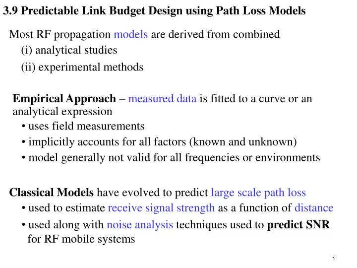
Classical Models have evolved to predict large scale path loss. used to estimate receive signal strength as a function of distance used along with noise analysis techniques used to predict SNR for RF mobile systems. 3.9 Predictable Link Budget Design using Path Loss Models.

E N D
Classical Models have evolved to predict large scale path loss • used to estimate receive signal strength as a function of distance • used along with noise analysis techniques used to predict SNR • for RF mobile systems 3.9 Predictable Link Budget Design using Path Loss Models • Most RF propagation models are derived from combined • (i) analytical studies • (ii) experimental methods • Empirical Approach – measured data isfitted to a curve or an • analytical expression • uses field measurements • implicitly accounts for all factors (known and unknown) • model generally not valid for all frequencies or environments
Ẽ = Ẽd Pr(d) = • Median Path Loss Determination • estimate receive power at distance d from transmitter Ẽ = total received electrical field (V/m) Ẽd = electric field of equivalent direct path N = number of paths between T and R Lk = relative loss of kth path k= relative phase shift of kth path if LOS exists L0= 1 and 0 = 0
3.9.1 Log Distance Path Loss Model • average received power decreases logarithmically with distance • theory & measurements indicate validity for indoors & outdoors (3.67) (3.68) (1) Average Large Scale Path Loss Model • distance dependentmean path loss - over significant distances d0= close in reference distance, often determined emperically d = transmitter - receiver separation n = path loss exponent - indicates rate of path loss increase with d0
Free Space Reference Distance, d0, • always in antenna’s far-field - eliminate near field effects for • reference path • must be specified for different environments • Reference Path Loss, PL(d0) calculated using either • (i) free space path loss (eqn 3.5) • (ii) field measurements at d0 Path Loss Exponent, n
PL(d) = (3.69a) PL(d) (dB) = (3.69b) Pr(d)(dB)= Pt(d) (dB) - PL(d) (dB) 3.9.2 Log Normal Shadowing • surrounding clutter isn’t considered by log distance model • averaged received power (eqn 3.68) is inconsistent with measured data • measured PL(d) at any location is random, with log normal distribution • about (normal distribution of log10(•) ) • antenna gains included in PL(d) • = zero-mean Gaussian distributed random variable (in dB) • = standard deviation of
f(xdB) = Pr[xdB = x] = it follows that Pr(xdB > x) = = • Log Normal Distribution - describes random shadowing effects • for specific Tx-Rx, measured signal levels have normal distribution • about distance dependent mean (in dB) • occurs over many measurements with same Tx-Rx & different • clutter standard deviation, (also measured in dB) • Lognormal Model For Local Shadowing • typically, dB ranges from 5-12 • let u = median path loss (dB) at distance d from transmitter • distribution xdB of observed path loss has pdf given by:
1 0.5 10-1 10-2 10-3 10-4 dB = 12 dB 8 dB 6 dB 4dB Pr (Gain < Abscissa) -12 -10 -8 -6 -4 -2 0 2 4 6 Gain relative to Median Path Loss(dB) • Log Normal Graph: Pr(xdB > x) vs Gain/Loss Relative to Median Path Loss • shown for dB = 4,6,8, 12 • median 50% of samples expected to be > median & • 50% expected to be < median • all curves intersect at median
Path Loss ModelParameters for arbitrary location & specified Tx-Rx • d0– close in reference distance • - clutter standard deviation • n – path loss exponent Used for system design & analysis simulations to provide estimated Pr(d)at random locations • & n are derived from measurements using linear regression • minimizes difference between measured & estimated path loss • minimized in a mean-square sense over many measurements & d’s
Q-function is used to determine probability that PR(d) threshold 3.70a where Q(-z) = 1- Q(z) 3.70b 3.71 • (i) PL(d) is RV with a normal distribution in dB about • as a result, Pr(d) inherits these characteristics Pr [Pr(d) > ]= Pr [Pr(d) < ]= 3.72 Q(z) = (ii) Pr(d) > or Pr(d) < is determined from CDF
U() = (3.73) U() = 3.9.3 Determination of % Coverage Area • in a given coverage area, let = desired receive signal level – • could be determined by receiver sensitivity (or visa versa) • random shadowing effects cause some locations at d to have • received power, Pr(d) < • Determine boundary coverage vs % area covered within a boundary, • assuming • a circular coverage area with radius R from base station • likelihood of coverage at cell boundary is known (given) • d = r represents radial distance from transmitter useful service area (coverage area): U() = % area with Pr(d) >
std deviation of path loss exponent /n = U() % Pr[Pr(r) > ] 1 0.95 0.90 0.85 0.80 0.75 0.70 0.65 0.60 0.95 0.90 0.85 0.80 0.75 0.70 0.65 0.60 0.55 0.50 0 1 2 3 4 5 6 7 8 /n Left Axis = % area with Pr(r) > (coverage area-use 3.73) Right Axis = Pr[Pr(r) > ] (boundary coverage-use 3.68)
3.10 Outdoor Propagation Model • estimating PL(d) requires terrain profilefor propagation over • irregular terrain such as • simple curved earth profile • highly mountainous • obstacles: trees, building, • all models predict Pr(d)at given point or small area (sector) • wide variations in approach, complexity, accuracy • most based on systematic interpretation of empirical data - Longely Rice - Durkins Model - Okumura Model - Hata Model - Wideband PCS Microcell - PCS Extension to Hata Model - Walfisch – Bertoni Model
(i) Median Transmission Loss predicted using path geometry of terrain profile & refractivity of troposphere • (ii)Signal Strengths within radio horizon predicted using Geometric Optics • Techniques (primarily 2-ray ground reflection) • (iii)Diffraction Loss over isolated obstacles predicted using Fresnel- • Kirchoff knife edge models • (iv) Troposcatter over long distances predicted using Forward Scatter • Theory • (v) Far-Field Diffractionlosses in double horizon paths predicted using • Modified Van der Pol-Bremner Method • 3.10.1 Longely Rice Model (ITS irregular terrain model) • used for point-point systems under different types of terrain • frequency ranges from 40MHz-100GHz
Longely Rice Model: available as a computer program • calculates large scale median transmission loss over irregular terrain for • frequencies between 20MHz-10GHz • input parameters include: • transmission frequency, • path length & antenna heights, • polarization, • surface refractivity • earth radius & climate • ground conductivity & ground dielectric constant • path specific parameters: antennas’ horizon distance, horizon elevation • angle, trans-horizon distance, terrain irregularity • Prediction Modes for Longely Rice • 1. point-point mode: used when detailed terrain profile or path • specific parameters are known • 2. area mode prediction: uses estimated path specific parameters
3.10.2 Durkins Model: similar to Longly-Rice • predicts field strength contours over irregular terrain • adopted by UK joint radio committee • consists of two parts • (1) ground profile • reconstructed from topographic data of proposed surface along • radial joining transmitter and receiver • models LOS & diffraction derived from obstacles & local scatters • assume all signal received along radial (no multipath) • (2) expected path loss calculated along the radial • move receiver location to deduce signal strength contour • pessimistic in narrow valleys • identifies weak reception areas well
3.10.3 Okumura Model – wholly based on measured data - no analytical explanation • among the simplest & best for in terms of path loss accuracy in • cluttered mobile environment • disadvantage: slow response to rapid terrain changes • common std deviations between predicted & measured path loss • 10dB - 14dB • widely used for urban areas • useful for • - frequencies ranging from 150MHz-1920MHz • - frequencies can be extrapolated to 3GHz • - distances from 1km to 100km • - base station antenna heights from 30m-1000m
Okumura developed a set of curves in urban areas with quasi-smooth terrain • effective antenna height: • - base station hte = 200m • - mobile: hre= 3m • gives median attenuation relative to free space (Amu) • developed from extensive measurements using vertical omni- • directional antennas at base and mobile • measurements plotted against frequency
Estimating path loss using Okumura Model • 1. determine free space loss, Amu(f,d), between points of interest • 2. add Amu(f,d) and correction factors to account for terrain L50(dB)= LF + Amu(f,d) – G(hte) – G(hre) – GAREA (3.80) L50 = 50% value of propagation path loss (median) LF = free space propagation loss Amu(f,d) = median attenuation relative to free space G(hte) = base station antenna height gain factor G(hre) = mobile antenna height gain factor GAREA = gain due to environment
Amu(f,d) & GAREA have been plotted for wide range of frequencies antenna gain varies at rate of 20dB per decade or 10dB per decade G(hte) = 10m < hte< 1000m (3.81a) hre 3m (3.81b) G(hre) = G(hre) = 3m < hre <10m (3.81b) • model corrected for • h = terrain undulation height • isolated ridge height • average terrain slope • mixed land/sea parameter
70 60 50 40 30 20 10 100 80 70 60 50 40 30 20 10 5 2 1 Urban Area ht= 200m hr= 3m d(km) Amu(f,d) (dB) 70 100 200 300 500 700 1000 2000 3000 f (MHz) Median Attenuation Relative to Free Space = Amu(f,d) (dB)
35 30 25 20 15 10 5 0 open area quasi open area suburban area GAREA(dB) 100 200 300 500 700 103 2103 3 103 frequency (MHz) Correction Factor = GAREA(dB)
3.10.4 Hata Model: empirical model of graphical path loss data from • Okumura • - predicts median path loss for different channels • - valid over UHF/VHF band from 150MHz-1.5GHz • - charts used to characterize factors affecting mobile land propagation • - standard formulas for approximating urban propagation loss • - correction factors for some situations • - compares closely with Okumura model as d > 1km large mobile • systems
(3.82) L50 (urban)(dB) = A + B log10d A= 69.55 + 26.16 log10(fc) – 13.82 log10(hte) – (hre) • represents fixed loss – approximately 2.6 power law dependence on fc • dependence on antenna heights is proportional to hre1.382 B= 44.9 - 6.55 log10(hte) • represents path loss exponent, worst case ≈ 4.5 • L50 (urban)(dB) = 69.55 + 26.16log10 fc– 13.82 log10 hte – (hre) • + (44.9-6.55hte)log10 d
Hata Model for Rural and Suburban Regions • represent reductions in fixed losses for less demanding environments Mobile Antenna Height Correction Factor for Hata Model
Valid Range for Parameters • 150MHz < fc < 1GHz • 30m < hb < 200m • 1m < hm < 10m • 1km < r < 20km • Propagation losses increase • with frequency • in built up areas
180 170 160 150 140 130 120 110 100 • hte = 30m • hre= 1m Path Loss (dB) 900 MHz 700 MHz 0 4 8 12 16 20 Range (km) 160 155 150 145 140 135 130 125 120 fc = 700MHz 20km 10km 5km Path Loss (dB) 20 60 100 140 180 hte (m) Example Tables for Okumura-Hata Model • Terrain Legend • Urban • Suburban • Open
(hre) defined in 3.83, 3.84a, 3.84b • for medium sized cities CM = 0dB • metropolitan centers CM = 3dB • 3.10.5 PCS Extension to Hata Model • European Co-operative Scientific & Technical (EUROCOST) • formed COST-231 • extend Hatas model to 2GHz L50 (urban)(dB) = 46.3 + 33.9logfc– 13.82 loghte – (hre) + (44.9-6.55hte)logd + CM fc = frequency from 1500MHz - 2 GHz hte = 30m-200m hre = 1m-10m d = 1km-20km
P0= (3.90) 3.10.6 Walfisch & Bertoni Model path loss: S = P0Q2P1 (3.89) P0 = free space path loss between isotropic antennas Q2 = reduction in rooftop signal due to row of buildings that immediately shadow hill P1 = based on diffraction determines signal loss from roof top to street S (dB) = L0 + Lrts + Lms (3.91) L0 = free space loss Lrts = roof-to-street diffraction & scatter loss Lms = multi-screen diffraction loss from rows of building
df = (3.92a) 3.10.7 Wideband PCS Microcell Model • FeuerstienMeasured cellular systems in Bay Area • - 20MHz pulsed transmitter at 1900 MHz • - base station antenna heights 3.7m, 8.5m, 13.3m • - mobile antenna heights 1.7m • assume flat ground reflection model • let df = 1st Fresnel zone clearance • Model for Average Path Loss - LOS channel • double regression model with regression breakpoint at 1st • Fresnel zone clearance • fits measured data well • model assumes omni-directional vertical antennas
(3.92b) p1 = = path loss in dB at reference distance d0 = 1m d = T-R separation distance n1, n2 = path loss exponents relates to antenna heights Average Path Loss – PCS Microcell e.g. at 1900MHz p1 = 38.0dB
= 10nlog(d) + p1 (3.92c) n = OBS path loss exponent – related to transmitter height = log normal shadowing component from distance dependent mean (3.10.2)
3.11 Indoor Propagation Model • smaller Tx-Rx separation distances than outdoors • higher environmental variability for much small Tx-Rx separation • - conditions vary from: doors open/closed, antenna position, • - variable far field radiation for receiver locations & antenna types • strongly influenced by building features, layout, materials • Dominated by same mechanisms as outdoor propagation (reflection, • refraction, scattering) • Classified as either LOS or OBS • Surveyed by [Mol91], [Has93] - Partition Losses – Same Floor - Partition Losses – Different Floor - Log-distance path loss model - Ericsson Multiple Breakpoint Model - Attenuation Factor Model
PL(dB) = (3.93) • Partition Losses – Same Floor • hard partitions: immovable, part of building • soft partitions: movable, lower than the ceiling Partition Losses – Different Floor: dependent on external building dimensions, structural characteristics & materials Log-distance path loss model: accurate for many indoor paths • n depends on surroundings and building type • = normal random variable in dB having std deviation • identical to log normal shadowing mode (3.69)
30 50 70 90 110 20dB attenuation (dB) 1 3 10 20 40 100 meters • (1) Ericsson Multiple Breakpoint Model: measurements in multi-floor office building • uses uniform distribution to generate path loss values between • minimum &maximum range, relative to distance • 4 breakpoints consider upper and lower bound on path loss • assumes 30dB attenutation at d0 = 1m • - accurate for f = 900MHz & unity gain anntenae • provides deterministic limit on range of path loss at given distance
3.94 PAF(1) PAF(2) FAF Rx Tx • (2) Attenuation Factor Model (Seidel92b) • includes effect of building type & variations caused by obstacles • reduces std deviation for path loss to 4dB • std deviation for path loss with log distance model 13dB • nSF = exponent value for same floor measurement – must be accurate • FAF = floor attenuation factor for different floor • PAF = partition attenuation factor for obstruction encountered by • primary ray tracing primary ray tracing = single ray drawn between Tx & Rx yields good accuracy with good computational efficiency
3.95 3.96 Replace FAF with nMF=exponent for multiple floor loss decreases as average region becomes smaller-more specific • Building Path Loss obeys free space + loss factor () (Dev90b) • loss factor increases exponentially with d • (dB/m) = attenuation constant for channel 4-story bldg 2-story bldg
Path Loss Exponent & Standard Deviation for Typical Building
Lp (dB) = (dB) + 2.47 (3) Simple Indoor Path Loss Model • r = distance between transmitter & receiver • r0 = nominal reference distance (typically 1m) • WAF(p) is wall attenuation factor, for P floors • FAF(q) is floor attenuation factor, for Q floors • n 2 for close distances, larger for greater distances • more accurate when P and Q are small • model neglects angle of incidence & effect of distance on n
3.12 Signal Penetration into Buildings • no exact models • signal strength increases with height • lower levels are affected by ground clutter (attenuation & • penetration) • higher floors may have LOS channel stronger incident signal on • walls • RF Penetration affected by • - frequency • - height within building • - antenna pattern in elevation plain
penetration loss • decreases with increased frequency • loss in front of windows is 6dB greater than without windows • penetration loss decreases 1.9dB with each floor when < 15th • floor • increased attenuation at >15 floors – shadowing affects from • taller buildings • metallic tints result in 3dB to 30dB attenuation • penetration impacted by angle of incidence
Penetration Loss vs Frequency for two different building (1) (2) • Ray Tracing & Site Specific Models • rapid acceleration of computer & visualization capabilities • SISP – site specific propagation models • GIS – graphical information systems • - support ray tracing • - augmented with aerial photos & architectural drawings