Download

1 / 37
370 likes | 455 Views
Using visibility as a surrogate for the trends of fine particle mass. Li Du. Visbility. Visibility is a good indicator of surface air quality and has the advantage of being easily obtained by observation.

E N D
Using visibility as a surrogate for the trends of fine particle mass Li Du
Visbility Visibility is a good indicator of surface air quality and has the advantage of being easily obtained by observation. Fine particles are efficient at scattering light and are strongly correlated with extinction coefficients, after correcting for meteorological conditions the potential and importance of using visibility as surrogate to the PM concentration distribution
PM2.5 = 7.6 g/m3 PM2.5 = 21.7 g/m3 PM2.5 = 65.3 g/m3 Adapted from Stephan’s report slides: Alternative Approaches for PM2.5 Mapping: Visibility as a Surrogate
Purpose of the study • explore the relationship between visibility ( extinction coefficient) and fine particle concentration • Use visibility datasets and the correlation to complement the PM distribution map especially for the region where PM monitoring are not systematically established
Visibility monitoring • Visibility has been serving for the airports and flights • In most of the countries, the visual range data is obtained by human observation • The stations are distributed over the world and data are more accessible
Extinction coefficient • Visual range observations provide a good indicator of air quality but have the disadvantage of being inversely related to aerosol concentrations. A more suitable measure is haziness or extinction coefficient K-Koshmieder constant
Databases • GSOD (Global summary of the day) -derived from data exchanged under World Meteorological Organization (WMO) World Weather Watch Program -contains 18 surface meteorological parameters derived from hourly observation, such as mean temperature, mean dew point -Flags are included for occurrence of snow, rain, hail, tornado and so on -visual range data obtained by human observers
Databases • ASOS (Automated Surface Observing System) - Starting from 1994-6, National Weather Services replaced human observers of visual range with automated light scattering instruments -measures the extinction coefficient on a one-min basis -ASOS package contains measurements of precipitation, temperature, dew point etc.
Comparison • GSOD • truncated data with lower precision; • threshold values of the visual range vary from sites to sites • daily averaged data may lose some information about the diurnal variation of aerosol concentration • Globally distributed stations and data started back to early 20th century
China India
Comparison ASOS • untruncated high-resolution data • detection threshold of scattering instrument is 0.05km-1 • not vulnerable to human observers’ subjectivity • Only started from 1994 and instrument measured data are available only in US
Visibility vs PM concentration Databases: GSOD-daily averaged human observed visibility data (humidity extinction coefficient, Bext) AQS_D: daily averaged ambient particle concentration; filter sample collected very third or sixth day Studied region: North America-US Latitude: 24~50 Longitude: -126~ -65 • There are no co-located ASOS and PM2.5 sites • The stations are not co-located but in the same city
Comparison of aggregated data Decide the time period during which the data are to be aggregated Choose the aggregation operator-75 percentile Compare the aggregated value of visibility and PM concentration in each corresponding grid Divide the studied region into m×n grids
Correlation between Bext and PM by aggregation from 2000 to 2005
Comparison between GSOD and AQS_D • The spatial pattern of visibility and PM distribution showed similarity in map • The worst correlation is observed to be in the winter (DJF), while the best correlation is observed to be in the summer (JJA). • The air in western US is quite pristine, and the visibility hits the threshold frequently. ---need high-resolution data and do single site comparison
ASOS dataset • ASOS Visibility Data Evaluation and Analysis -a project conducted during 2001 and 2002 1. evaluate the quality of ASOS data; 2.explore the relationship between ASOS visibility and hourly PM data and seek for the potential of using visibility as PM surrogate
ASOS Bext Threshold: 0.05 km-1 • The Bext values below 0.05 km-1 are reported as 0.05. • Based on Koschmieder, the ASOS lower detection limit is ~ 50 mile visual range • In the pristine SW US, the ASOS threshold distorts the data • However over the East and Western US, the Bext signal is well over the detection limit
Typical Diurnal Pattern of Bext, Temperature and Dewpoint • Typically, Bext shows a strong nighttime peak due to high relative humidity. • Most of the increase is due to water absorption by hygroscopic aerosols. At RH >90% , the aerosol is mostly water • At RH < 90%, the Bext is mostly influenced by the dry aerosol content; the RH effect can be corrected. Adapted from R. Husar’s report slides Macon, GA, Jul 24, 2000
Adopted RH Correction Curve RH is calculated fromT – Temperature, deg C and D – Dewpoint, deg C RH = 100*((112-(0.1*T)+D)/(112+(0.9*T)))8 Correction factor: C=8E-08*RH^4-7E-06*RH^3+0.0003*RH^2-0.0032*RH+1.0046 Adopted from Evaluation of the Light Scattering Data from the ASOS Network(ppt) by Rudolf B Husar
RH correction Adopted from Evaluation of the Light Scattering Data from the ASOS Network(ppt) by Rudolf B Husar
Correlation over US Greensburg, NC Pensacola, FL Albuquerque, NM Odessa, TX
Diurnal Cycle of Relative Humidity and Bext The diurnal RH cycle causes the high Bext values in the misty morning hours The shape of the RH-dependence is site (aerosol) dependent Relative Humidity Bext
Summary • The extinction coefficient is quite humidity dependence, and the dependence is not uniform • The relationship is heterogeneous over the US, but whether it is highly regional is still to be work out • Using visibility as surrogates for PM is meaningful in eastern US, but questionable in the western and southwestern US • Humidity correction to the available visibility data is quite important. Specific correction curve are to be studied for each region