Download
1 / 57
580 likes | 777 Views
Numerical Modeling for Flow and Transport. P. Bedient and A. Holder Rice University 2005. Uses of Modeling. A model is designed to represent reality in such a way that the modeler can do one of several things:

E N D
Numerical Modeling for Flow and Transport P. Bedient and A. Holder Rice University 2005
Uses of Modeling • A model is designed to represent reality in such a way that the modeler can do one of several things: • Quickly estimate certain aspects of a system (screening models, analytical solutions, ‘back of the envelope’ calculations) • Determine the causes of an observed condition (flow direction, contamination, subsidence, flooding) • Predict the effects of changes to a system (pumping, remediation, development, waste disposal)
Types of Ground Water Flow Models • Analytical Models (Exp and ERF functions) • 1-D solution, Ogata and Banks (1961) • 2-D solution, Wilson and Miller (1978) • 3-D solutions, Domenico & Schwartz (1990) • Numerical Models (Solved over a grid - FDE) • Flow-only models in 3-D (MODFLOW) • MODPATH - allows tracking of particles in 2-D placed in flow field produced from MODFLOW
Governing Equation for Flow • For two-dimensional transient flow conditions • Transient means that the water level changes with time • Steady state means it is constant in time. • S = storativity [unitless], • Q = recharge or withdrawal per unit area [L/T] • T = transmissivity [L2/T]
Poisson’s Equation • The basic flow equation in a homogeneous, confined, 2-D aquifer at steady-state (S = 0), with sources and/or sinks • Can be solved analytically or numerically • Theis’ Analytical solution in cylindrical coordinates • Gauss-Seidel with Successive Over-Relaxation (SOR)
Laplace’s Equation • If there are no source/sink terms, Poisson’s equation reduces to Laplace’s Equation • Can also be solved analytically or numerically • Gauss-Seidel Iteration method • Successive Over Relaxation method • Solutions are generally smooth and well-behaved
Numerical Solutions • For complex layered, heterogeneous aquifers, a numerical approximation is required in non-uniform flow • Several types — Finite Difference, Finite Element, and Method of Characteristics • Finite difference approximations involve applying Taylor’s expansions to the equations (flow and transport) and approximating the derivatives in the equation • Other methods involve different approximations, but all are based generally on the Taylor expansion
Taylor’s Expansion from Calculus Taylor’s Series provides a means to predict a function f(x) value at one point in terms of a function value and its derivatives at another point. Zero Order approximation might be f(xi+1) = f(xi) Value at new point is same as at old point First Order approximation is f(xi+1) = f(xi) + f’(xi)(xi+1 – xi) Straight line projection to next point Second Order approximation captures curvature f(xi+1) = f(xi) + f’(xi)(xi+1 – xi) + f’’(xi) (xi+1 – xi)2 2!
Approximation of f(x) by various orders f(x) Zero Order First Order Second Order True Fcn Xi Xi+1 DX
Taylor’s Expansion from Calculus Any function h(x) can be expressed as an infinite series: Where h’(x) is the first derivative and h’’(x) is the second derivative and so on.
Taylor’s Expansion for Second Derivative Adding the above two eqns, and neglecting all the higher terms, and rearranging terms gives a useful approximation for h’’(x) : True Function h(x) h(x - Dx) h(x) h(x + Dx)
Taylor’s Expansion for dh/dx Neglecting second and all higher powers, and rearranging terms gives a forward or backward difference approximation for the first derivative or h’(x) : Forward Diff Backward Diff True Function h(x) h(x - Dx) h(x) h(x + Dx)
Numerical Soln to Laplace’s Equation DX hi,j • Assume ∆x = ∆y [regular square grid] • Represent h(xi,yj) = hi,j • h(xi+∆x, yj+∆y) = hi+1,j+1, Thus replacing terms in Laplace, the F.D.E. becomes • Do the same for the ‘j’ direction, and you have the following: DY yj+1 yj yj-1 xi-1 xi xi+1
Approximation to Laplace’s Eqn. Summing terms and solving for hi,j gives:
h = 0 1 2 h = 0 h = 0 3 4 h = 1 Application to a Simple 3x3 Grid • Start with boundary conditions and initial estimate for h, assume h1 = h2 = h3 = h4 = 0 • Get a new estimate for h1, call it h1m+1 • h1m+1 = (top + right + bottom + left)/4 • h1m+1 = {0 + h2 + h3 + 0}/4 • Repeat four internal points - 2, 3, and 4 using same four-star average calculation
h = 0 1 2 h = 0 h = 0 3 4 h = 1 Application to a grid h1m+1 = {0 + h2m + h3m + 0 } /4 h2m+1 = {0 + 0 + h4m + h1m} /4 h3m+1 = {h1m + h4m + 1 + 0 } /4 h4m+1 = {h2m + 0 + 1 + h3m} /4 • Use the initial values and boundary conditions for the first approximation • Use the updated values (m+1) for further approximations (m+2) • Continue until the numbers don’t change much (convergence!)
Convergence Criteria • Convergence for a flow code requires that the change in the solution at each point be less than a specified target, called the convergence criterion, or sometimes epsilon, • If is too large, convergence will occur before a solution is reached • If is too small, convergence may take very long, or be impossible due to oscillation • There is more than one way to define convergence, including global measures, local measures, etc.
Gauss-Seidel Method • Uses partially completed iteration to estimate values for the rest of the iteration. • h1m+1 = {0 + h2m + h3m + 0 }/4 • h2m+1 = {0 + 0 + h4m + h1m}/4 • h3m+1 ={h1m+1 + h4m + 1 + 0 }/4 • h4m+1 ={h2m+1 + 0 + 1 + h3m}/4 • Use m+1update iteration values for h1 and h2 when computing h3 and h4 • Results in faster convergence over a large grid
Successive Over-Relaxation - SOR • To speed up the convergence, overshoot the standard model. • Defining the Residual, c = hi,jm+1* – hi,jm • Using: hi,jm+1 = hi,jm + c = (1–) hi,jm + hi,jm+1*, where is the relaxation factor and hi,jm+1* is given by the Gauss-Seidel approximation, we get: • hi,jm+1=(1-)hi,jm +(/4)(hi-1,jm+1 + hi,j-1m+1 + hi+1,jm + hi,j+1m ) • If = 1, reduces to Gauss-Seidel • If 1 < < 2, the method is over-relaxed - usually ~ 1.4 - 1.5
Numerical Simulation Models Numerical models solve approximations of the governing equations of flow and transport - over a grid system • Based on a grid or mesh laid over the study site • Helps organize large datasets into logical units • Data required includes boundary conditions, hydraulic conductivity, thickness, pump rates, recharge, etc.) • Can be computationally intensive • Can be applied to actual field sites to help understand complex hydrogeologic interrelationships.
Often-Used Numerical Models MODFLOW (1988) - USGS flow model for 3-D aquifers MODPATH - flow line model for depicting streamlines MOC (1988) - USGS 2-D advection/dispersion code MT3D (1990, 1998) - 3-D transport code works with MODFLOW RT3D (1998) - 3-D transport chlorinated - MODFLOW BIOPLUME II, III (1987, 1998) - authored at Rice Univ 2-D based on the MOC procedures.
Numerical Solution of Equations Numerically -- H or C is approximated at each point of a computational domain (may be a regular grid or irregular) • Solution is very general • May require intensive computational effort to get the desired resolution • Subject to numerical difficulties such as convergence problems and numerical dispersion • Generally, flow and transport are solved in separate independent steps (except in density-dependent or multi-phase flow situations)
MODFLOW Introduction • Written in the 1984 and updated in 1988 • Solves governing equations of flow for a full 3-D aquifer system with variable K, b, recharge, drains, rivers, and pumping wells. • Withdrawal and injection wells (rates may change with time) • Constant head boundaries or regions (ponds/rivers/fixed heads) • No-flow boundaries or regions (bedrock outcrops/water divides) • Regions of diffuse recharge or discharge (rainfall) • Observation wells
MODFLOW MODFLOW is a modular 3-D finite-difference flow code developed by the U.S. Geological Survey to simulate saturated flow through a layered porous media. The PDE solved is for h(x,y,z,t): • where Kxx, Kyy, and Kzz are defined as the hydraulic conductivity along the x, y, and z coordinate axis, h represents the potentiometric head, W is the volumetric flux per unit volume being pumped, Ss is the specific storage of the porous material and t is time.
MODFLOW Features • MODLOW consists of a main program and a series of independent subroutines grouped into packages. • Each package controls with a specific feature of the hydrologic system, such as wells, drains, and recharge. The division of the program into packages allows the user to analyze the specific hydrologic feature of the model independently.
MODFLOW Features • MODFLOW is one of the most versatile and widely accepted groundwater models • It is particularly good in heterogeneous regions because it allows for vertical interchange between layers, as well as horizontal flow within the aquifers. • It also allows for variable grids to speed computation. • It has been applied to model thousands of field sites containing a number of different contaminants and for a number of different remediation applications.
Solution Methods • MODFLOW is an iterative numerical solver (SIP or SOR). • The initial head values are provided and the these heads are gradually changed through a series of time steps, in the case of a transient model run, until the governing equation is satisfied. Time steps can be variable to speed output. • The primary output from the model is the head distribution in x, y, and z, which can then be used by a transport model. • In addition, a volumetric water budget is provided as a check on the numerical accuracy of the simulation.
MODFLOW - Input to Transport Models • Designed to create modern GUI to ease large data entry and output graphical manipulation for applications to complex field sites • GMS - 1995 • Visual MODFLOW • Ground Water Vistas PLUME visualization
MODPATH - Pathlines • Designed to use heads from MODFLOW and linear interpolation to compute velocity Vx and or Vy. • Particles can be placed in areas of known or suspected source concentrations in order to create possible tracks of contaminants in space and time - streaklines Path results after two time steps
MODPATH • Designed to use heads from MODFLOW and linear interpolation to compute velocity Vx in the x direction: • Vx = (1-fx)Vx(i -1/2) +fxVx(i +1/2) • Where fx = (xp - x(i-1/2) / Dxi,j • And xp is the x coordinate of the particle Particle Location In Grid i, j (i - 1/2, j) (i + 1/2, j) Vx Dx
10 yr pathlines Wei 03 2-layer final elev(Weifinal) Dec 2002 Original
MODPATH - EXAMPLE • Designed to create modern GUI to ease large data entry and output graphical manipulation for applications to complex field sites Source
Alternative 3 Alternative 2
Alternative 4 Alternative 3 Alternative 2
Contaminant Transport in 2-D C = Concentration of Solute [M/L3] DIJ = Dispersion Coefficient [L2/T] - x and y B = Thickness of Aquifer [L] C’ = Concentration in Sink Well [M/L3] W = Flow in Source or Sink [L3/T] E = Porosity of Aquifer [unitless] VI = Velocity in ‘I’ Direction [L/T] - x and y
Domenico and Schwartz (1990) • 3-D solutions for several geometries (listed in Bedient et al. 1999, Section 6.8) - spreadsheets exist • Generally a vertical plane, constant concentration source.
Method of Characteristics USGS (MOC) • Written for USGS by Konikow and Bredehoeft in 1978 • Solves flow equations with Alternating Direction Implicit (ADI) method • Solves transport equations via particle tracking method and finite difference • Using velocities calculated from the flow solution, vx = kx(∆h/∆x), particles are moved • Concentrations are based on the average concentration of all particles in a cell at the end of the time step Velocity
MOC Concepts • Partial Differential Equation replaced by equivalent set of ODEs called ‘characteristic equations’ (approximated with finite difference) • Particle in a cell is moved a distance proportional to the seepage velocity within the cell • Accounts for concentration change due to advection • Remainder of governing equation solved by finite difference methods • Accounts for concentration change due to dispersion, changes in saturated thickness, and fluid sources
MOC/BIOPLUME II Capabilities • Can simulate effects of natural or enhanced biodegradation: • Fast-equilibrium biodegradation • First-order biodegradation • Monod kinetics • Withdrawal and injection wells (pump and treat systems) • Injection wells for oxygen enhancement • Observation wells within and outside plume area