Download
1 / 92
940 likes | 1.12k Views
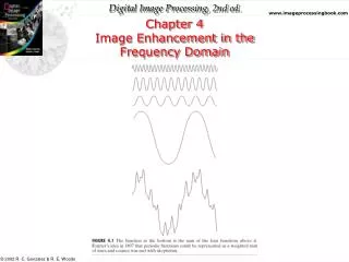
Chapter 4 Image Enhancement in the Frequency Domain. 國立雲林科技大學 電子工程系 張傳育 (Chuan-Yu Chang ) 博士 Office: ES 709 TEL: 05-5342601 ext. 4337 E-mail: chuanyu@yuntech.edu.tw. Background. Fourier series:

E N D
Chapter 4Image Enhancement in the Frequency Domain 國立雲林科技大學 電子工程系 張傳育(Chuan-Yu Chang ) 博士 Office: ES 709 TEL: 05-5342601 ext. 4337 E-mail: chuanyu@yuntech.edu.tw
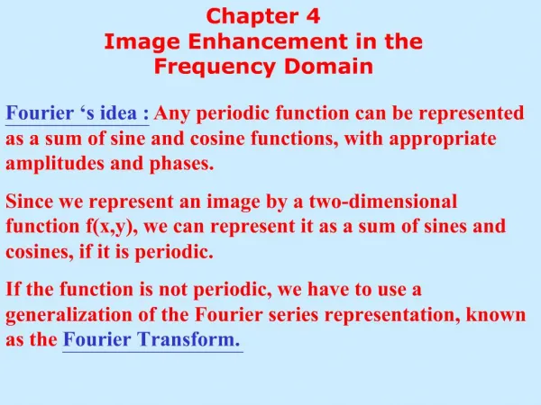
Background • Fourier series: • Any function that periodically repeats itself can be expressed as the sum of sines and/or cosines of different frequencies, each multiplied by a different coefficient • Fourier transform • Even functions that are not periodic can be integral of sines and/or cosine multiplied by a weighting function. • A function expressed in either a Fourier series or transform, can be reconstructed completely via an inverse process, with no loss of information.
The 1D Fourier Transform Fourier Transform Pair (4.2-1) and (4.2-2) • The Fourier transform, F(u), of a single variable, continuous function, f(x), is defined as • We can obtain f(x) by means of the inverse Fourier transform • Extended to two variables, u and v. (4.2-1) (4.2-2) A function can be recovered from its transform. (4.2-3) (4.2-4)
The 1D Fourier Transform (cont.) 在離散FT時,乘數所放的位置並不重要,可放在轉換前或轉換後,或者兩個都放,但須滿足其乘積為1/M • Discrete Fourier Transform, DFT • The concept of the frequency domain follows directly from Euler’s Formula • Substituting (4.2-7) into (4.2-5) obtain DFT: (4.2-5) (4.2-6) IDFT: (4.2-7) (4.2-8) 每一分項稱為頻率成分(frequency component) Each term of the Fourier Transform is composed of the sum of all values of the function f(x).
The 1D Fourier Transform (cont.) • Glass prism • The prism is a physical device that separates light into various color components, each depending on its wavelength content. • The Fourier transform • The FT may be viewed as a “mathematical prism” that separates a function into various components, based on frequency content. • The Fourier transform lets us characterize a function by its frequency content.
The 1D Fourier Transform (cont.) • As in the analysis of complex numbers, we find it convenient sometimes to express F(u) in polar coordinates Rear part of F(u) imaginary part of F(u) (magnitude, spectrum) (phase angle, phase spectrum) (power spectrum, spectral density)
Example 4.1: Fourier spectra of two simple 1-D function • 在x域曲線下的面積加倍時,頻譜上的高度也會加倍。(The height of the spectrum doubled as the area under the curve in the x-domain doubled.) • 當函數長度加倍時,在相同區間上頻譜的零點加倍。(The number of zeros in the spectrum in the same interval doubled as the length of the function doubled) A=1,K=8,M=1024
The 1D Fourier Transform (cont.) • 處理離散變數時,可以下式表示函數f(x) • 同理,因為頻率總是由零頻率開始,因此F(u) • Fig. 4.2顯示,f(x)和F(u)成倒數關係 (4.2-13) (4.2-14) (4.2-15)
The 1D Fourier Transform (cont.) • In the discrete transform of Eq(4.2-5), the function f(x)for x=0, 1, 2,…,M-1, represents Msamples from its continuous counterpart. • These samples are not necessarily always taken at integer values of x in the interval [0, M-1]. They are taken at equally spaced. • Let x0denote the first point in the sequence. The first value of the sampled function is f(x0). The next sample has taken a fixed interval Dx units away to give f(x0+Dx). The k-th sample is f(x0+kDx). • The sequence always starts at true zero frequency. Thus the sequence for the values of u is 0, Du, 2Du,…,[M-1]Du. The F(u) • Dx and Du are inversely related by the expression (in Fig. 4.2) (4.2-13) (4.2-14) (4.2-15)
The 2D DFT and Its Inverse • 2D DFT pair (4.2-16) (4.2-17) 2D Fourier spectrum, phase angle, power spectrum (4.2-18) (4.2-19) (4.2-20)
The 2D DFT and Its Inverse • It is common practice to multiply the input image function by (-1)x+y prior to computing the Fourier transform. (4.2-21) Shifts the origin of F(u,v) to frequency coordinates(M/2,N/2), which is the center of the MxN area occupied by the 2-D DFT. This area of the frequency domain is called Frequency rectangle
The 2D DFT and Its Inverse (cont.) • The value of the transform at (u,v)= (0,0) is • F(0,0) sometimes is called the dc component of the spectrum. • If f(x,y) is real, its Fourier transform is conjugate symmetric (4.2-22) (4.2-23) The spectrum of the Fourier transform is symmetric. (4.2-24) (4.2-25) (4.2-26)
Example 4.2:Centered spectrum of a simple 2-D function The image was processedprior to displaying by using the log transformation in Eq.(3.2-2) White rectangle of size 20x40 pixels The image was multiplied by (-1)x+y prior to computing the Fourier transform
Filtering in the Frequency domain • Some basic properties of the frequency domain • Frequency is directly related to rate of change. • The slowest varying frequency component (u=v=0) correspond to the average gray level of an image. • As we move away from the origin of the transform, the low frequencies correspond to the slowly varying components of an image. • As we move further away from the origin of the transform, the higher frequencies correspond to the faster and faster gray level changes in the image.
Filtering in the Frequency domain (cont.) • In spatial domain • g(x,y)=h(x,y)*f(x,y) • In frequency domain • H(u,v) is called a filter. • The Fourier transform of the output image is • G(u,v)=H(u,v)F(u,v) • The filtered image is obtained simply by taking the inverse Fourier transform of G(u,v) • Filtered Image=F-1[G(u,v)] The multiplication of H and F involves two-dimensional functions and is defined on an element-by-element basis.
Filtering in the Frequency domain (cont.) Basics of filtering in the frequency domain • Multiply the input image by (-1)x+y to center the transform • Compute F(u,v), the DFT of the image from (1) • Multiply F(u,v) by a filter function H(u,v) • Compute the inverse DFT of the result in (3) • Obtain the real part of the result in (4) • Multiply the result in (5) by (-1)x+y
Filtering in the Frequency domain (cont.) • Basic steps for filtering in the frequency domain
Some basis filters and their properties • Notch filter • It is a constant function with a hole at the origin. • Set F(0,0) to zero and leave all other frequency components of the Fourier transform untouched.
Example • Result of filtering the image in Fig. 4.4(a) with a notch filter that set to 0 the F(0,0) term in the Fourier transform. • In reality the average of the displayed image cannot be zero because the image has to have negative values for its average gray level to be zero and displays cannot handle negative quantities. • The most negative value was set to zero, and other values scaled up from that.
Some basis filters and their properties • Low frequencies in Fourier transform are responsible for the general gray-level appearance of an image over smooth areas. • High frequencies are responsible for detail, such as edges and noise. • A filter that attenuates high frequencies while passing low frequencies is called a low pass filter. • A lowpass-filtered image has less sharp detail than original image. • A filter that has the opposite characteristic is called a high pass filter. • A highpass-filtered image has less gray level variations in smooth areas and emphasized transitional gray-level detail. • Such an image will appear sharper.
The effects of lowpass and highpass filtering Blurred image Lowpass Sharp image withlittle smooth graylevel detail becausethe F(0,0) has beenset to zero. Highpass
Example • Result of highpass filtering the image in Fig. 4.4(a) The highpass filter is modified by adding a constant of one-half the filter height to the filter function
Correspondence between Filtering in the Spatial and Frequency Domains • Convolution theorem (4.2-30) • Flipping one function about the origin. • Shifting that function with respect to the other by changingthe values of (x,y) • Computing a sum of products over all values of m and n,for each displacement (x,y).
Correspondence between Filtering in the Spatial and Frequency Domains (cont.) Used to indicate that the expression on the left can be obtained by taking the IFT of the expression on the right. • Fourier transform pair • Impulse function of strength A (4.2-31) (4.2-32) (4.2-33) (4.2-34) (位於原點的單位脈衝)
Correspondence between Filtering in the Spatial and Frequency Domains (cont.) • The Fourier transform of a unit impulse at the origin • Let f(x,y)=d(x,y), Eq.(4.2-30) and (4.2-34) (4.2-35) (4.2-36)
Correspondence between Filtering in the Spatial and Frequency Domains (cont.) • Based on (4.2-31), combining (4.2-35) and (4.2-36) • Given a filter in the frequency domain, we can obtain the corresponding filter in the spatial domain by taking the IFT of the former. • We can specify filters in the frequency domain, take their inverse transform, and then use the resulting filter in the spatial domain as a guide for constructing smaller spatial filter masks. (4.2-37)
Introduction to the Fourier Transform and the Frequency Domain (cont.) • 高斯濾波器(Gaussian Filter) • The corresponding filter in the spatial domain • These two equations represent an important result for two reasons: • They constitute a Fourier transform pair, both components of which are Gaussian and real. (上述二式構成Fourier transform pair,兩個成分均為高斯且為實數。) • These functions behave reciprocally with respect to one another. (這些函數彼此互為倒數。) • 當H(u)有較大範圍的剖面時,h(x)有較窄的剖面。
Introduction to the Fourier Transform and the Frequency Domain (cont.) • We can construct a highpass filter as a difference of Gaussians, as follows: • With A>=B and s1>s2. • The corresponding filter in the spatial domain is
Introduction to the Fourier Transform and the Frequency Domain (cont.) Once the values turn negative, they never turn positive again. We can implement lowpass filtering in the spatial domain by using a mask with all positive coefficients.
Smoothing Frequency-Domain Filters • Ideal Low-pass Filter • 2 D ideal lowpass filter • Cuts off all high frequency components of the FT that are at a distance greater than a specified distance D0 from the origin of the transform. 從點(u,v)到傅立葉轉換中心點的距離 (4.3-2) (4.3-3)
Smoothing Frequency-Domain Filters (cont.) • 截止頻率(cutoff frequency) • H(u,v)=1和H(u,v)=0之間的過渡點。 • 整體功率(total image power) • Summing the components of the power spectrum at each point (u,v). • 百分比功率(% of the power) (4.3-4) (4.3-5)
Example 4.4 Image power as a function of distance from the origin of the DFT 半徑為5, 15, 30, 80, and 230 功率比為92, 94.6, 96.4, 98, and 99.5
Example 4.4 Image power as a function of distance from the origin of the DFT (cont.) 存在振鈴現象(ringing)
Smoothing Frequency-Domain Filters (cont.) • 巴特沃斯特低通濾波器(Butterworth Lowpass Filter) • BLPF transfer function does not have a sharp discontinuity (BLPF沒有銳利不連續的截止頻率) • Defining a cutoff frequency locus at points for which H(u,v) is down to a certain fraction of its maximum value. (將截止頻率定義在H(u,v)降到最大值的某個比例時。)
Smoothing Frequency-Domain Filters (cont.) • 一階的BLPF沒有振鈴也沒有負值。 • 二階的BLPF有輕微的振鈴,有小負值。 • 高階的BLPF有明顯的振鈴,
Smoothing Frequency-Domain Filters (cont.) • The BLPF of order 1 has neither ringing nor negative values. • The filter of order 2 does show mild ringing and small negative values, but they certainly are less obvious than in the ILPF. • Ringing in the BLPF becomes significant for higher-order filter.
Smoothing Frequency-Domain Filters (cont.) • 高斯低通濾波器(Gaussian Lowpass Filters) • Let s=D0, • where D0 is the cutoff frequency.
Smoothing Frequency-Domain Filters (cont.) • Example 4.6: Gaussian lowpass filtering • A smooth transition in blurring as a function of increasing cutoff frequency. • No ringing in the GLPF.
Smoothing Frequency-Domain Filters (cont.) • A sample of text of poor resolution • Using a Gaussian lowpass filter with
Smoothing Frequency-Domain Filters (cont.) • A sample of text of poor resolution • Using a Gaussian lowpass filter with D0=80 to repair the text.
Smoothing Frequency-Domain Filters (cont.) • Cosmetric processing • Appling the lowpass filter to produce a smoother, softer-looking result from a sharp original. • For human faces, the typical objective is to reduce the sharpness of fine skin lines and small blemishes.
Smoothing Frequency-Domain Filters (cont.) • (a) High resolution radiometer image showing part of the Gulf of Mexico (dark) and Folorida (light). • Existing many horizontal sensor scan lines. • (b) After Gaussian lowpass filter with D0=30. • (c) After Gaussian lowpass filter with D0=10. • The objective is to blur out as much detail as possible while leaving large features recognizable.
Sharpening Frequency Domain Filters • Edges and other abrupt changes in gray levels are associated with high-frequency components. • Image sharpening can be achieved in the frequency domain by a highpass filtering process. • Attenuating the low frequency components without disturbing high-frequency information in the Fourier transform. • The transform function of the highpass filters can be obtained using the relation
Sharpening Frequency Domain Filters • 理想高通濾波器(Ideal Highpass Filters) • 巴特沃斯高通濾波器(Butterworth Highpass Filters) • 高斯高通濾波器 (Gaussian Highpass Filters) (4.4-2) (4.4-3) (4.4-4)
Sharpening Frequency Domain Filters (cont.) It set to zero all frequencies inside a circle of radius D0 while passing without attenuation, all frequencies outside the circle. The IHPF is not physically realizable with electronic components, but it can be implemented in a computer.
Sharpening Frequency Domain Filters (cont.) • Spatial representations of typical (a) ideal (b) Butterworth, and (c) Gaussian frequency domain highpass filters
Sharpening Frequency Domain Filters (cont.) • Result of ideal highpass filtering (a) with D0=15, 30, and 80 • IHPFs have ringing properties.
Sharpening Frequency Domain Filters (cont.) • Result of BHPF order 2 highpass filtering (a) with D0=15, 30, and 80