Download
1 / 26
260 likes | 400 Views
Sorting out GRB correlations with spectral peak David Eichler (presented by Jonathan Granot ). Hypothesis: GRB spectra are intrinsically similar – peaking at ~ 1 MeV , & the apparent differences are due to viewing angle effects. .

E N D
Sorting out GRB correlations with spectral peak David Eichler (presented by Jonathan Granot)
Hypothesis: GRB spectra are intrinsically similar – peaking at ~ 1 MeV, & the apparent differences are due to viewing angle effects.
Eiso- peak correlation(Amati et al 2002, Atteia et al 2003) Eiso peak2
Observer outside of extended beam – offset angle less than or comparable to opening angle of beam - sees diminished Eiso and npeak as per the Amati et al. relation, However, there must be many such viewers. So consider a beam shape that accommodates many such viewers by having lots of perimeter relative to solid angle….e.g. annulus.
Off-axis Viewing as Grand Eiso- peak Correlate Viewer outside annulus annulus Pencil beam Eichler & Levinson (2004)
Inside annulus Epeak -1, Eiso -where 1+(obs)2 2 for/2< |obs-0|≲ 0(near edge) 3 for obs≳ 20 (point source limit) Eichler & Levinson (2004)
Choosing an annulus with half-opening angle 0 0.1 rad, thickness 0.03 rad, and G ~ 102, and standard cosmology gives a distribution of (cosmological redshift uncorrected) Epeak that is flat, as observed (Eichler & Levinson 2004).
“on-axis” events at redshifts where most of the comoving volume resides obsfrom the jet symmetry axis at the maximal redshift out to which it could be detected (XRFs) “Off-axis” (GRBs) “on-axis” Different jet thicknesses Eichler & Levinson (2004)
Different fluence detection thresholds XRF’s GRB’s 10 KeV 1 MeV
Why is the Ghirlanda relation, Eg (Epeak )1.5, different from the Amati relation, Eiso (Epeak)2?
If afterglow theory is correct, INFERRED opening angle is overestimated for off-beam viewing by p1/4. This explains the p1/2 difference between the Amati and Ghirlanda relations Levinson and Eichler (2005). Eiso = fb-1E(Ep/Ep,max)- , fb (out2-in2)/2, 2 jet = 0.16[tjet,d/(1+z)]3/8(n0/Eiso,52)1/8 (Eiso)-1/8 fb,app jet2/2 out2/2 (Eiso)-1/4 Ep- /4 E,app = fb,appEiso [1- (in/out)2]-1E(Ep/Ep,max)-3/4
Eisopeak2 (Amati et al 2002, Atteia et al 2003) Epeak1.5 (Ghirlanda et. al 2004)
= K tb3/8Ek,iso-1/8, then the beaming correction, q2 is proportional to Ek,iso-1/4 or npeak1/2. • So the true opening angle is confirmed, within the framework of this interpretation, to indeed be • Ek,iso-1/8, as predicted by afterglow theory.
So, with the viewing angle interpretation, everybody should be happy. Amati et al. and Ghirlanda et al. should both be happy because they are both right. Frail et al should be happy that an additional effect, besides opening angle correction, explains residual dispersion in Eiso.
Afterglow theorists should be happy that break times are connected to opening angle. AND that the true opening angle is indeed “measured” to be proportional to Ek,iso-1/8. Viewing angle proponents should be happy that no ad hoc intrinsic dependence of npeak needs to be invoked to understand Amati et al relations and the like.
Why is X-ray afterglow almost always seen within several hours? Because the 1/G beaming cone of the afterglow emission cone is wider, after several hours, than that of the prompt emission, and is wide enough to cover most relevant viewing angles.
Off-beam viewer sees slower decline (or possibly rise) in the X-ray afterglow light curve (compared to an on-beam viewer) during the first several minutes to hours.
Gamma ray efficiencies (i.e. gamma ray energy to blast energy)
Plotting gamma ray efficiency Eg/EB– gamma ray energy to inferred blast energy - with and without viewing angle correction shows a qualitative difference in the ordering of the data. (Eichler & Jontof-Hutter 2005) With the viewing angle correction the gamma rayefficiencies separate into two classes. The majority (17/22) has Eg/EB ~ 7
The other - 5 outliers of total sample of 22 GRB’s with known redshifts - has Eg/EB ~102. Note that all outliers have Eg/EB >> 1. No outliers in the other direction yet.
Without viewing angle correction, the scatter in gamma ray efficiency is much larger
Implications of the viewing angle interpretation: • Most of the energy is in gamma rays. Only ~15% of the energy is in the afterglow shock. Gamma rays may energize baryons rather than the reverse. • Sometimes only ~10-2 of the total energy is in the forward shock (baryon-poor line of sight?) • Intrinsic spectrum peaks at ~1 MeV, as expected from a pair annihilation photosphere (Levinson & Eichler 1999). • Non-simple jet topology (e.g. annulus) gives best fit to data.