Download
1 / 47
520 likes | 927 Views
Free-Form Deformations. Free-Form Deformation of Solid Geometric Models Fast Volume-Preserving Free Form Deformation Using Multi-Level Optimization Free-Form Deformations with Lattices of Arbitrary Topology. Introduction - Bezier Curves. Control Polygon Parametric Equations

E N D
Free-Form Deformations Free-Form Deformation of Solid Geometric Models Fast Volume-Preserving Free Form Deformation Using Multi-Level Optimization Free-Form Deformations with Lattices of Arbitrary Topology
Introduction - Bezier Curves • Control Polygon • Parametric Equations • Weighting Functions • De Casteljau Subdivision
Control Polygon • Bezier Curve is defined by a set of n points (in 1D, 2D, 3D, etc) • order • weight • degree • The points (in order) joined by lines is called the Control Polygon P4 P3 P2 P1
Parametric Equations • Each of the points on the Bezier Curve is defined as functions of t • in 3D x(t), y(t), z(t) • These functions are based on the points of the control polygon (P1…Pn)
Weighting Functions • Bernstein Polynomials • x(t) = Σ(i=0..n)(ni) (1-t)n-i ti Pix • This must be evaluated for t = 0..1 at the resolution desired • This must also be evaluated for each variable of the space (x, y, z in 3D)
De Casteljau Subdivision(aka Better Intuition) • t = 0.5: P4 P3 P2 P1
Picture Pages • Time to get your crayons and your pencils!
Higher Dimensions • Bezier Curves are considered 1D objects because only one variable changes (t) • However, higher spaces exist for Bezier arithmetic and FFDs take advantage of these multivariate spaces
Remainder of Talk • Free-Form Deformation of Solid Geometric Models • Sederberg and Parry - SIGGRAPH 1986 • Faster and Volume Preserving Free Form Deformation Using Multi-Level Optimization • Hirota, Maheshwari, and Lin – ACM Solid Modelling • Free-Form Deformations with Lattices of Arbitrary Topology • MacCracken and Joy – SIGGRAPH 1996
This Section • Free-Form Deformation of Solid Geometric Models • Sederberg and Parry - SIGGRAPH 1986 • Faster and Volume Preserving Free Form Deformation Using Multi-Level Optimization • Hirota, Maheshwari, and Lin – ACM Solid Modelling • Free-Form Deformations with Lattices of Arbitrary Topology • MacCracken and Joy – SIGGRAPH 1996
Free-Form Deformation • Redefine any form of 3D data into trivariate Bernstein Polynomial basis • (x, y, z) (s, t, u) • Alter trivariate control polygon • Solve for altered 3D vertices • (s, t, u) (x’, y’, z’)
2D Example 1 *(Approximate) Q4 Q3 Q1x= -1 Q1s= .2 Q2x= 1 Q2s= .8 .75 Q3x= 1 Q3s= .8 Q4x= -1 Q4s= .2 t= .25 Q1 Q2 0 0 .25 .75 1 s=
2D Example (cont) 1 *(Approximate) Q1s= .2 Q1x= -.7 Q2s= .8 Q2x= 1 .75 Q3s= .8 Q3x= 1 t= Q4s= .2 Q4x= -1 .25 0 0 .25 .75 s= 1
Demo • My Implementation of 3D-FFD
Why is this useful? • Any primitive may be placed in Control Mesh • Basic Primitives may be molded into complex shapes, joined with guaranteed continuity • Volume may be preserved
Outline • Free-Form Deformation of Solid Geometric Models • Sederberg and Parry - SIGGRAPH 1986 • Faster and Volume Preserving Free Form Deformation Using Multi-Level Optimization • Hirota, Maheshwari, and Lin – ACM Solid Modelling • Free-Form Deformations with Lattices of Arbitrary Topology • MacCracken and Joy – SIGGRAPH 1996
Goal of Volume Preservation • Deformations are more physically accurate when volume is preserved • Fixed position for some portion of deformation • Alter location of remaining portions according to an energy minimization scheme
V2 V3 Axy = (V1V2xV1V3)z 2 V1 h = (V1z+V2z+V3z) 3 Calculating Volume • In a closed manifold approximated by a polygonal mesh: • Volume = Axy*h
Calculating Volume 2 • For back-facing polygons Volume is negative • Benefits • Translation independent • Really fast • Can be used to recompute the normals after deformation
Modifying Volume • After a deformation, the volume of the solid has changed • Some control points are locked down and a minimization must be performed
Energy Minimization • The lattice is considered a spring system • This becomes a minimization problem: • Min Espring(X) • Subject to ΔV(X) = 0 • X is the Matrix of the Control Point Positions
Equations • Espring(X)=Σjk/2(sqrt((Xej-Xsj)(Xej-Xsj))–Lj)2 • Note that sqrt(x2) is abs(x) • However, left in this form to show the equation is “well over quartic” • We need to differentiate E and V • dV/dX = dV/dP* dP/dX • We can solve for dP/dX and dV/dP quickly
Iterative Refinement • This is best solved iteratively • Refined answer obtained after each step • To increase speed of calculation smaller polygonal meshes used at first
Iterative Refinement 3 • λ = Lagrange multiplier • σ = penalty for volume deviation
Finally • Free-Form Deformation of Solid Geometric Models • Sederberg and Parry - SIGGRAPH 1986 • Faster and Volume Preserving Free Form Deformation Using Multi-Level Optimization • Hirota, Maheshwari, and Lin – ACM Solid Modelling • Free-Form Deformations with Lattices of Arbitrary Topology • MacCracken and Joy – SIGGRAPH 1996
General Deformations • FFD can not easily handle all forms of deformation • Lattices are constrained to parallel-piped • This paper allows for a more general definition of deformation space
Lattice Definition • Edge – two vertices connected in the simplicial complex • Face – minimal connected loop of vertices • Cell – region bounded by a set of faces
Catmull-Clark Subdivision 1 • face point - the average of all of the points defining the original face. • edge point - the average of the midpoint of original edge with two new, neighboring face points. • vertex point - (Q + 2R + (n-3)V_i)/n • Q is the average of the face points containing V_i • R is the average of the midpoints of the edges incident to V_i • n is the number of faces containing V_i. • Images and text taken from http://www.math.tuwien.ac.at/~gkneisl/Recent_Work/Thesis.html
Catmull-Clark Subdivision 2 • Expanded here for use in volumes: • Cell Point (Ci)– Average of vertices in the lattice • Face Point (Fi) – (C0+2A+C1)/4 • Edge Point (Ei) – (Cavg+2Aavg+(n-3)M)/4 • Vertex Point (Vi) – (Cavg+3Aavg+3Mavg+P)/8 • Ai is a “Face Centroid”
Added “Special Cases” • In order to allow for better volume matching, corner vertices and sharp edges are defined specially
Calculating s,t,u • Subdivide volume a small number of times • Calculate “relative” s,t,u in the current cell
Deformation Process • Deform Control Lattice • Subdivide to necessary size • Calculate new xyz position
What you should know • FFD is by far the easier, faster concept • Volume Preservation can best be done by hierarchical refinement • More general deformations can be defined • Numerical methods must be employed • Greater user input required for lattice construction