LCFR Water Quality Modeling Project Report

1. LCFR Water Quality ModelingProject Report Jim Bowen, UNC Charlotte LCFRP Advisory Board/Tech. Comm. Meeting, October 30, 2008 Raleigh, NC

2. Outline of Presentation • A Quick Review of the LCFR Model • Summary of Model Report • Questions/Suggestions

3. Basis of PresentationTechnicalReportDraft(available on web)

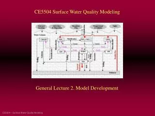
4. LCFR Dissolved Oxygen ModelThe big picture “Met” Data Air temps, precip, wind, cloudiness Hydrologic Conditions River Flows, Temp’s, Conc’s Tides Time Estuary Physical Characteristics: e.g. length, width, depth, roughness Time EFDC Software Adjustable Parameters: (e.g. BOD decay, SOD, reaeration) State Variables nutrients DO, organic C Time

5. Dissolved Oxygen Conceptual ModelBOD Sources Cape Fear, Black & NECF BOD Load decaying phytopl. Estuary Inflow BOD Load Muni & Ind. BOD Load Sediment

6. Dissolved Oxygen Conceptual ModelBOD Sources, DO Sources Cape Fear, Black & NECF BOD Load decaying phytopl. Surface Reaeration Estuary Inflow BOD Load Phytoplank. Productivity Muni & Ind. BOD Load Ocean Inflows MCFR Inflows Sediment

7. Dissolved Oxygen Conceptual ModelBOD Sources, DO Sources & Sinks Input of NECF & Black R. Low DO Water Cape Fear, Black & NECF BOD Load decaying phytopl. Surface Reaeration Estuary Inflow BOD Load Phytoplank. Productivity Muni & Ind. BOD Load BOD Consumption Ocean Inflows MCFR Inflows Sediment Sediment O2 Demand

8. Steps in Applying a Mechanistic Model • Decide on What to Model • Decide on Questions to be Answered • Choose Model • Collect Data for Inputs, Calibration • Create Input Files • Create Initial Test Application • Perform Qualitative “Reality Check” Calibration & Debugging

9. Steps in Applying a Mechanistic Model, continued • Perform quantitative calibration & model verification • Design model scenario testing procedure (endpoints, scenarios, etc.) • Perform scenario tests • Assess model reliability • Document results

10. Description of Model Application Black River Flow Boundary Cond. NE Cape Fear Flow Boundary Cond. Cape Fear R. Flow Boundary Cond. Lower Cape Fear River Estuary Schematic Open Boundary Elevation Cond.

11. Description of Model Application • Flow boundary condition upstream (3 rivers) • Elevation boundary condition downstream • 20 lateral point sources (WWTPs) • Extra lateral sources add water from tidal creeks, marshes (14 additional sources) • 37 total freshwater sources

12. Model State Variables • Water Properties • Temperature, salinities • Circulation • Velocities, water surface elevations • Nutrients • Organic and inorganic nitrogen, phosphorus, silica • Organic Matter • Organic carbon (labile particulate, labile and refractory dissolved), phytoplankton (3 groups) • Other • Dissolved oxygen, total active metal, fecal coliform bacteria

13. Water Quality Model Schematic

14. Data Collected to Support Model • Data Collected from 8 sources • US ACoE, NC DWQ, LCFRP, US NOAA, US NWS, USGS, Wilmington wastewater authority, International Paper • Nearly 1 TB of original data collected • File management system created to save and protect original data

15. Observed Data Used to Create Model Input Files • Meteorological forcings (from NWS) • Freshwater inflows (from USGS) • Elevations at Estuary mouth (from NOAA) • Quality, temperature of freshwater inflows and at estuary mouth (from LCFRP, USGS, DWQ) • Other discharges (from DWQ)

16. EFDC Input Files & Data Sources

17. Lower Cape Fear River Program Sites Used

18. USGS Continuous Monitoring and DWQ Special Study Stations Used

19. New Cross- Sections Surveyed by NC DWQ

20. SOD Monitoring Stations Performed by NC DWQ

21. LCFR Grid • Channel Cells in Blue • Wetland Cells in White • Marsh and Swamp Forest in Green, Purple

22. LCFR Grid Characteristics • Grid based on NOAA bathymetry and previous work by TetraTech • Off-channel storage locations (wetland cells) based on wetland delineations done by NC DCM • 1050 total horizontal cells (809 channel cells, 241 wetland cells) • 8 vertical layers for each horizontal cell • Used a sensitivity analysis to locate and size wetland cells

23. Model Grid Showing Location and Size of Wetland Cells

24. Riverine Swamps and Saltwater Marshes in Estuary (NC DCM)

25. Input File Specification • Inflows • Temperatures and Water Quality Concentrations at Boundaries • Water quality mass loads for point sources • Benthic fluxes • Meteorological data

26. Riverine Inflow Specification • Flows based on USGS flow data • Flows scaled based upon drainage area ratios • 17 total inflows • 3 rivers, 14 estuary sources

27. Subwatersheds Draining Directly to the Estuary

28. Subwatersheds Draining Directly to the Estuary

29. Temperature and Concentration Specification • 5 stations used (3 boundaries, 2 in estuary) • Combined USGS and LCFRP data • Point source specification tied to closest available data

30. Use data interpolation and estimation to create a monitoring data set with no data gaps, enter data into Excel spreadsheet, one spreadsheet for each source For each source, create a data conversion matrix to estimate each model constituent from the available parameters in the source data For source data given as a concentration time history, multiply concentrations by flows to get mass loads Collect mass load time histories and reformat, then write into WQPSL.INP file using Matlab script Procedure for creating water quality mass load file (WQPSL.INP) • Used an automated procedure based upon available data (LCFRP, DMR’s)

31. An Example Conversion Matrix (Cape Fear River Inflow)

32. Benthic fluxes and meteorological data • Used a prescriptive benthic flux model • SODs time varying, but constant across estuary • SOD values based upon monitoring data • Met data constant across estuary • Met data taken from Wilmington airport

33. Model Calibration and Confirmation • 2004 calendar year used for model calibration • Nov 1, 2003 to Jan. 1 2004 used for model startup • 2005 calendar year used for confirmation run (a.k.a. verification, validation run)

34. Streamflows during Model Runs • 2004 dry until October • Early 2005 had some high flows • Summer 2005 was dry

35. Hydrodynamic Model Calibration • Examined water surface elevations, temperatures, salinities • Used LCFRP and USGS data for model/data comparisons of salinity temperature • Used USGS and NOAA data for model/data comparisons of water surface elevation • USGS data based on pressure measurements not corrected for barometric changes

36. Monitoring Stations Used for Hydrodynamic Calibration

37. Simulation of Tidal Attenuation in Estuary • Varied wetland cell widths to determine effect on attenuation of tidal amplitude • Wider wetland cells gave more attenuation, as expected • Also tried different distribution of wetland cells within estuary

38. M2 Tidal Amplitude for Various Cell Width Scenarios

39. M2 Tidal Amplitude for Various Cell Distribution Scenarios

40. M2 Tidal Amplitude for Various Cell Distribution Scenarios Width * 2, v1 chosen as best overall (in green)

41. Example Time Series Comparison – Black at Currie (upstream), 2004

42. Example Time Series Comparison – NECF at Wilmington, 2004

43. Example Time Series Comparison – Cape Fear at Marker 12, 2004

44. Example Time Series Comparison – Black at Currie (upstream), Jan. 04

45. Example Time Series Comparison – Wilm. Tide Gage, Jan. 04

46. Example Time Series Comparison – Cape Fear at Marker 12, Jan. 04

47. Example Time Series Comparison – Salinities at Navassa, 2004

48. Example Time Series Comparison – Salinities at NECF Wilm., 2004

49. Example Time Series Comparison – Salinities at Marker 12, 2004

50. Calibration Statistics, Salinity