Download
1 / 19
190 likes | 193 Views
An Extensible Global Address Space Framework with Decoupled Task and Data Abstractions *. Sriram Krishnamoorthy Jarek Nieplocha Umit Catalyurek Atanas Rountev P. Sadayappan The Ohio State University Pacific Northwest Natl. Lab.

E N D
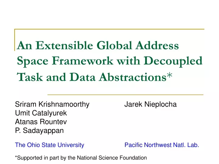
An Extensible Global Address Space Framework with Decoupled Task and Data Abstractions* Sriram Krishnamoorthy Jarek Nieplocha Umit Catalyurek Atanas Rountev P. Sadayappan The Ohio State UniversityPacific Northwest Natl. Lab. *Supported in part by the National Science Foundation
Theory #Terms #F77Lines Year CCD 11 3209 1978 CCSD 48 13213 1982 CCSDT 102 33932 1988 CCSDTQ 183 79901 1992 Time Crunch in Quantum Chemistry Two major bottlenecks in computational chemistry: • Very computationally intensive models (performance) • Extremely time consuming to develop codes(productivity) The vicious cycle in many areas of computational science: • More powerful computers make more and more accurate models computationally feasible :-) • But efficient parallel implementation of complex models takes longer and longer • Hence computational scientists spend more and more time with MPI programming, and less time actually doing science :-( • Coupled Cluster family of models in electronic structure theory • Increasing number of terms => explosive increase in code complexity • Theory well known for decades but efficient implementation of higher-order models took many years
CCSD Doubles Equation (Quantum Chemist’s Eye Test Chart :-) hbar[a,b,i,j] == sum[f[b,c]*t[i,j,a,c],{c}] -sum[f[k,c]*t[k,b]*t[i,j,a,c],{k,c}] +sum[f[a,c]*t[i,j,c,b],{c}] -sum[f[k,c]*t[k,a]*t[i,j,c,b],{k,c}] -sum[f[k,j]*t[i,k,a,b],{k}] -sum[f[k,c]*t[j,c]*t[i,k,a,b],{k,c}] -sum[f[k,i]*t[j,k,b,a],{k}] -sum[f[k,c]*t[i,c]*t[j,k,b,a],{k,c}] +sum[t[i,c]*t[j,d]*v[a,b,c,d],{c,d}] +sum[t[i,j,c,d]*v[a,b,c,d],{c,d}] +sum[t[j,c]*v[a,b,i,c],{c}] -sum[t[k,b]*v[a,k,i,j],{k}] +sum[t[i,c]*v[b,a,j,c],{c}] -sum[t[k,a]*v[b,k,j,i],{k}] -sum[t[k,d]*t[i,j,c,b]*v[k,a,c,d],{k,c,d}] -sum[t[i,c]*t[j,k,b,d]*v[k,a,c,d],{k,c,d}] -sum[t[j,c]*t[k,b]*v[k,a,c,i],{k,c}] +2*sum[t[j,k,b,c]*v[k,a,c,i],{k,c}] -sum[t[j,k,c,b]*v[k,a,c,i],{k,c}] -sum[t[i,c]*t[j,d]*t[k,b]*v[k,a,d,c],{k,c,d}] +2*sum[t[k,d]*t[i,j,c,b]*v[k,a,d,c],{k,c,d}] -sum[t[k,b]*t[i,j,c,d]*v[k,a,d,c],{k,c,d}] -sum[t[j,d]*t[i,k,c,b]*v[k,a,d,c],{k,c,d}] +2*sum[t[i,c]*t[j,k,b,d]*v[k,a,d,c],{k,c,d}] -sum[t[i,c]*t[j,k,d,b]*v[k,a,d,c],{k,c,d}] -sum[t[j,k,b,c]*v[k,a,i,c],{k,c}] -sum[t[i,c]*t[k,b]*v[k,a,j,c],{k,c}] -sum[t[i,k,c,b]*v[k,a,j,c],{k,c}] -sum[t[i,c]*t[j,d]*t[k,a]*v[k,b,c,d],{k,c,d}] -sum[t[k,d]*t[i,j,a,c]*v[k,b,c,d],{k,c,d}] -sum[t[k,a]*t[i,j,c,d]*v[k,b,c,d],{k,c,d}] +2*sum[t[j,d]*t[i,k,a,c]*v[k,b,c,d],{k,c,d}] -sum[t[j,d]*t[i,k,c,a]*v[k,b,c,d],{k,c,d}] -sum[t[i,c]*t[j,k,d,a]*v[k,b,c,d],{k,c,d}] -sum[t[i,c]*t[k,a]*v[k,b,c,j],{k,c}] +2*sum[t[i,k,a,c]*v[k,b,c,j],{k,c}] -sum[t[i,k,c,a]*v[k,b,c,j],{k,c}] +2*sum[t[k,d]*t[i,j,a,c]*v[k,b,d,c],{k,c,d}] -sum[t[j,d]*t[i,k,a,c]*v[k,b,d,c],{k,c,d}] -sum[t[j,c]*t[k,a]*v[k,b,i,c],{k,c}] -sum[t[j,k,c,a]*v[k,b,i,c],{k,c}] -sum[t[i,k,a,c]*v[k,b,j,c],{k,c}] +sum[t[i,c]*t[j,d]*t[k,a]*t[l,b]*v[k,l,c,d],{k,l,c,d}] -2*sum[t[k,b]*t[l,d]*t[i,j,a,c]*v[k,l,c,d],{k,l,c,d}] -2*sum[t[k,a]*t[l,d]*t[i,j,c,b]*v[k,l,c,d],{k,l,c,d}] +sum[t[k,a]*t[l,b]*t[i,j,c,d]*v[k,l,c,d],{k,l,c,d}] -2*sum[t[j,c]*t[l,d]*t[i,k,a,b]*v[k,l,c,d],{k,l,c,d}] -2*sum[t[j,d]*t[l,b]*t[i,k,a,c]*v[k,l,c,d],{k,l,c,d}] +sum[t[j,d]*t[l,b]*t[i,k,c,a]*v[k,l,c,d],{k,l,c,d}] -2*sum[t[i,c]*t[l,d]*t[j,k,b,a]*v[k,l,c,d],{k,l,c,d}] +sum[t[i,c]*t[l,a]*t[j,k,b,d]*v[k,l,c,d],{k,l,c,d}] +sum[t[i,c]*t[l,b]*t[j,k,d,a]*v[k,l,c,d],{k,l,c,d}] +sum[t[i,k,c,d]*t[j,l,b,a]*v[k,l,c,d],{k,l,c,d}] +4*sum[t[i,k,a,c]*t[j,l,b,d]*v[k,l,c,d],{k,l,c,d}] -2*sum[t[i,k,c,a]*t[j,l,b,d]*v[k,l,c,d],{k,l,c,d}] -2*sum[t[i,k,a,b]*t[j,l,c,d]*v[k,l,c,d],{k,l,c,d}] -2*sum[t[i,k,a,c]*t[j,l,d,b]*v[k,l,c,d],{k,l,c,d}] +sum[t[i,k,c,a]*t[j,l,d,b]*v[k,l,c,d],{k,l,c,d}] +sum[t[i,c]*t[j,d]*t[k,l,a,b]*v[k,l,c,d],{k,l,c,d}] +sum[t[i,j,c,d]*t[k,l,a,b]*v[k,l,c,d],{k,l,c,d}] -2*sum[t[i,j,c,b]*t[k,l,a,d]*v[k,l,c,d],{k,l,c,d}] -2*sum[t[i,j,a,c]*t[k,l,b,d]*v[k,l,c,d],{k,l,c,d}] +sum[t[j,c]*t[k,b]*t[l,a]*v[k,l,c,i],{k,l,c}] +sum[t[l,c]*t[j,k,b,a]*v[k,l,c,i],{k,l,c}] -2*sum[t[l,a]*t[j,k,b,c]*v[k,l,c,i],{k,l,c}] +sum[t[l,a]*t[j,k,c,b]*v[k,l,c,i],{k,l,c}] -2*sum[t[k,c]*t[j,l,b,a]*v[k,l,c,i],{k,l,c}] +sum[t[k,a]*t[j,l,b,c]*v[k,l,c,i],{k,l,c}] +sum[t[k,b]*t[j,l,c,a]*v[k,l,c,i],{k,l,c}] +sum[t[j,c]*t[l,k,a,b]*v[k,l,c,i],{k,l,c}] +sum[t[i,c]*t[k,a]*t[l,b]*v[k,l,c,j],{k,l,c}] +sum[t[l,c]*t[i,k,a,b]*v[k,l,c,j],{k,l,c}] -2*sum[t[l,b]*t[i,k,a,c]*v[k,l,c,j],{k,l,c}] +sum[t[l,b]*t[i,k,c,a]*v[k,l,c,j],{k,l,c}] +sum[t[i,c]*t[k,l,a,b]*v[k,l,c,j],{k,l,c}] +sum[t[j,c]*t[l,d]*t[i,k,a,b]*v[k,l,d,c],{k,l,c,d}] +sum[t[j,d]*t[l,b]*t[i,k,a,c]*v[k,l,d,c],{k,l,c,d}] +sum[t[j,d]*t[l,a]*t[i,k,c,b]*v[k,l,d,c],{k,l,c,d}] -2*sum[t[i,k,c,d]*t[j,l,b,a]*v[k,l,d,c],{k,l,c,d}] -2*sum[t[i,k,a,c]*t[j,l,b,d]*v[k,l,d,c],{k,l,c,d}] +sum[t[i,k,c,a]*t[j,l,b,d]*v[k,l,d,c],{k,l,c,d}] +sum[t[i,k,a,b]*t[j,l,c,d]*v[k,l,d,c],{k,l,c,d}] +sum[t[i,k,c,b]*t[j,l,d,a]*v[k,l,d,c],{k,l,c,d}] +sum[t[i,k,a,c]*t[j,l,d,b]*v[k,l,d,c],{k,l,c,d}] +sum[t[k,a]*t[l,b]*v[k,l,i,j],{k,l}] +sum[t[k,l,a,b]*v[k,l,i,j],{k,l}] +sum[t[k,b]*t[l,d]*t[i,j,a,c]*v[l,k,c,d],{k,l,c,d}] +sum[t[k,a]*t[l,d]*t[i,j,c,b]*v[l,k,c,d],{k,l,c,d}] +sum[t[i,c]*t[l,d]*t[j,k,b,a]*v[l,k,c,d],{k,l,c,d}] -2*sum[t[i,c]*t[l,a]*t[j,k,b,d]*v[l,k,c,d],{k,l,c,d}] +sum[t[i,c]*t[l,a]*t[j,k,d,b]*v[l,k,c,d],{k,l,c,d}] +sum[t[i,j,c,b]*t[k,l,a,d]*v[l,k,c,d],{k,l,c,d}] +sum[t[i,j,a,c]*t[k,l,b,d]*v[l,k,c,d],{k,l,c,d}] -2*sum[t[l,c]*t[i,k,a,b]*v[l,k,c,j],{k,l,c}] +sum[t[l,b]*t[i,k,a,c]*v[l,k,c,j],{k,l,c}] +sum[t[l,a]*t[i,k,c,b]*v[l,k,c,j],{k,l,c}] +v[a,b,i,j]
Tensor Contraction Engine • Automatic transformation from high-level specification • Chemist specifies computation in high-level mathematical form • Synthesis system transforms it to efficient parallel program • Code is tailored to target machine • Code can be optimized for specific molecules being modeled • Multi-institutional collaboration (OSU, LSU, U. Waterloo, ORNL, PNNL, U. Florida) • Prototypes of TCE are operational • a) Full functionality but fewer optimizations (So Hirata, PNNL), b) Partial functionality but more sophisticated optimizations • Already used to implement new models, included in latest release of NWChem • First parallel implementation for many of the methods • Significant interest in quantum chemistry community • Built on top of the Global Arrays parallel library range V = 3000; range O = 100; index a,b,c,d,e,f : V; index i,j,k : O; mlimit = 10000000; function F1(V,V,V,O); function F2(V,V,V,O); procedure P(in T1[O,O,V,V], in T2[O,O,V,V], out X)= begin A3A == sum[ sum[F1(a,b,e,k) * F2(c,f,b,k), {b,k}] * sum[T1[i,j,c,e] * T2[i,j,a,f], {i,j}], {a,e,c,f}]*0.5 + ...; end
Physically distributed data Global Address Space Global Arrays Library Distributed dense arrays that can be accessed through a shared view single, shared data structure with global indexing e.g.,accessA(4,3) rather than Alocal(1,3) on process 4
Shared Object copy to shared object put compute/update local memory local memory local memory Global Array Model of Computations Shared Object copy to local memory get • Shared memory view for distributed dense arrays • MPI-Compatible; Currently usable with Fortran, C, C++, Python • Data locality and granularity control similar to message passing model • Used in large scale efforts, e.g. NWChem (million+ lines/code)
Parochiality 3 P’s of Parallel Programming ParadigmsPerformance Productivity Parochiality “Holy Grail” TCE GA MPI OpenMP Performance Autoparallelized Productivity C/Fortran90
Pros and Cons of the GA Model • Advantages • Provides convenient global-shared view, but the get-compute-put model ensures user focus on data-locality optimization => good performance • Inter-operates with MPI to enable general applicability • Limitations • Only supports dense multi-dimensional arrays • Data view more convenient than MPI, but computation specification is still “process-centric” • No support for load balancing of irregular computations
Main Ideas in Approach Proposed • Decoupled task and data abstractions • Layered, multi-level data abstraction • Global-shared view highly desirable, but efficient word-level access to shared data infeasible (latency will always be much larger than 1/bandwidth) => chunked access • Lowest abstraction layer: Globally addressable “chunk” repository • Multi-dimensional block-sparse array is represented as a collection of small dense multi-dimensional bricks (chunks) • Bricks are distributed among processors; globally addressable and efficiently accessible • Computation Abstraction • Non-process-specific collection of independent tasks • Only non-local data task can access: parts of global arrays (patches of dense GA’s or bricks of block-sparse arrays) • Task-data affinity is modeled as a hypergraph; hypergraph partitioning used to achieve • Locality-aware load balancing • Transparent access to in-memory versus disk-resident data
Hypergraph Formulation for Task Mapping • Vertices • One per task, weight = computation cost • Hyper-edges • One per data brick, weight = size of brick (Communication cost) • Connects tasks that access brick • Hypergraph partitioning to determine task mapping • Pre-determined distribution for data bricks (e.g. round-robin on hash) • Zero-weight vertex for each data brick, “pinned” to predetermined processor
Example C = A * B Array B 3 3 3 3 3 2 3 3 3 Array C 3 3 2 Array A
* = Tasks: [c-brick, a-brick, b-brick] [0x0, 0x0, 0x0] [0x0, 0x1, 1x0] [0x1, 0x0, 0x1] [0x1, 0x1, 1x1] [1x0, 1x0, 0x0] [1x0, 1x1, 1x0] [1x1, 1x0, 0x1] [1x1, 1x1, 1x1] [4x4, 4x2, 2x4] [4x4, 4x3, 3x4] [2x2, 2x4, 4x2] [2x3, 2x4, 4x3] [3x2, 3x4, 4x2] [3x3, 3x4, 4x3] [5x5, 5x5, 5x5]
27 27 [0x1, 0x0, 0x1] [0x0, 0x0, 0x0] 0 72 0 0x1 0x1 72 0x0 27 0x0 [0x1, 0x1, 1x1] 27 [0x0, 0x1, 1x0] 27 27 0 [4x4, 4x2, 2x4] [1x1, 1x0, 0x1] 4x4 0 72 72 1x1 1x1 4x4 27 [1x1, 1x1, 1x1] 27 27 [1x0, 1x0, 0x0] [4x4, 4x3, 3x4] 0 72 0 1x0 1x0 27 72 27 2x2 2x2 [2x2, 2x4, 4x2] [1x0, 1x1, 1x0] 0 3x3 0 0 72 27 5x5 2x3 2x3 [2x3, 2x4, 4x3] 32 72 5x5 3x3 0 27 72 8 27 3x2 3x2 [3x2, 3x4, 4x2] [5x5, 5x5, 5x5] [3x3, 3x4, 4x3]
Transparent Memory Hierarchy Management • Problem: Schedule computation and disk I/O operations • Objective: Minimize disk I/O • Constraint: Memory limit constraint • Solution: Hypergraph partitioning formulation • Efficient solutions to the hypergraph problem exist • Typically used in the context of parallelization • Number of parts known • No constraints such as memory limit • Only balancing constraint
Hypergraph Formulation for Memory Management • Formulation • Tasks -> vertices • Data -> Nets • No pre-assignment of nets to certain parts • Balance: Memory usage in the parts • Guarantees solution for some #parts, if it exists • Determine dynamically #parts • Modify the inherent recursive procedure of hypergraph partitioning.
Read-Once Partitioning • Direct solution to above problem • Similar to approaches to parallelization • No refined reuse relationships • All tasks within a part have reuse, and none outside • Read-Once Partitioning • Group tasks into steps • Identify data common across steps and load into memory • For each step, read non-common (step-exclusive) data, process tasks, and write/discard step-exclusive data • Better utilization of memory available -> reduced disk I/O
Read-Once Partitioning: Example Disk I/O: 8 data elements Disk I/O: 9 data elements
Related Work • Sparse or block-sparse matrices in parallel libraries supporting sparse linear algebra • Aztec, PETSc etc. • Load-balancing • Work-stealing - Cilk • Object migration – Charm++ • Dynamic scheduling of loop iterations – OpenMP • Unaware of runtime systems support for: • Flexible global-shared abstractions for semi-structured data • Locality-aware, load-balanced scheduling of parallel tasks • Transparent access to in-memory and disk-resident data
Summary and Future Work • Summary • Global-shared abstraction and distributed implementation on clusters, for multi-dimensional block-sparse arrays • Locality-aware load balancing of tasks operating on block-sparse arrays • Ongoing/Future Work • Improve performance through overlapping communication with computation • Transparent extension of global-shared data/computation abstraction for “out-of-core” case • Extension of the approach for oct-tree and other data structures – target application: multi-wavelet quantum chemistry code recently developed by Robert Harrison at ORNL