Download
1 / 14
140 likes | 147 Views
Section 7.2 Tables 7.2-1 and 7.2-2 summarize hypothesis tests about one mean. (These tests assume that the sample is taken from a normal distribution, but the tests are robust when the sample is taken from a non-normal distribution with finite mean and variance.)

E N D
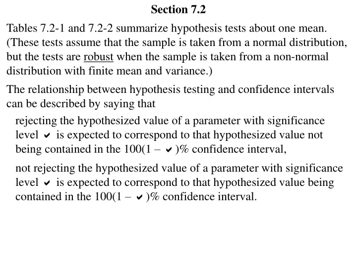
Section 7.2 Tables 7.2-1 and 7.2-2 summarize hypothesis tests about one mean. (These tests assume that the sample is taken from a normal distribution, but the tests are robust when the sample is taken from a non-normal distribution with finite mean and variance.) The relationship between hypothesis testing and confidence intervals can be described by saying that rejecting the hypothesized value of a parameter with significance level is expected to correspond to that hypothesized value not being contained in the 100(1 – )% confidence interval, not rejecting the hypothesized value of a parameter with significance level is expected to correspond to that hypothesized value being contained in the 100(1 – )% confidence interval.
Confidence intervals have the following properties: (1) (2) Hypothesis tests have the following properties: (1) (2) For fixed sample size n, the length of the confidence interval tends to be __________ as the confidence level 100(1 – )% is increased, and the length of the confidence interval tends to be __________ as the confidence level 100(1 – )% is decreased. larger smaller For fixed confidence level 100(1 – )%, the length of the confidence interval tends to be __________ as the sample size n is increased, and the length of the confidence interval tends to be __________ as the sample size n is decreased. smaller larger For fixed sample size n, as the significance level is decreased, a type II error probability is __________, and as the significance level is increased, a type II error probability is __________. increased decreased For fixed significance level , as the sample size n is increased, a type II error probability is __________, and as the sample size n is decreased, a type II error probability is __________. decreased increased
1. It is assumed that the cereal weight in a “10-ounce box” is N(, 2). To test H0: = 10.1 versus H1: > 10.1 with a 0.05 significance level, a random sample of size n = 16 boxes is selected where it is observed that x = 10.4 and s = 0.4. (a) Calculate the appropriate test statistic, describe the appropriate critical region, and write a summary of the results. x– 10.1 ——— = s /n 10.4 – 10.1 ————— = 0.4 /16 3.000 The test statistic is t = The one-sided critical region with = 0.05 is t1.753 . Since t = 3.000 > t0.05(15) = 1.753, we reject H0. We conclude that the mean weight of cereal per box is greater than 10.1 ounces.
(b) Find the approximate p-value of this hypothesis test. The p-value of the test is a t(15) random variable X– 10.1 ——— 3.000; = 10.1 = S /n P P(T 3.000) is slightly less than 0.005.
2. (a) Use the Analyze > Compare Means > One-Sample T Test options in SPSS to do Text Exercise 7.2-4. x– 7.5 ——— = s /n x– 7.5 ——— s /10 The test statistic is t = The two-sided critical region with = 0.05 is |t| 2.262 . – 2.262 2.262 = t0.025(9)
(b) From the SPSS output, we find t = 1.539 .
Since t = 1.539 < t0.025(9) = 2.262, we fail to reject H0. We conclude that the mean thickness for vending machine spearmint gum is not different from 7.5 hundredths of an inch. (c) From the SPSS output, we find that the limits of the 95% confidence interval for are 7.4765 and 7.6235. The hypothesized mean = 7.5 is contained in these limits, just as we would expect. Note that to calculate the p-value of this test, we need to find X– 7.5 ——— 1.539; = 7.5 S /n P
3. (a) (b) (c) (d) Use the Analyze > Compare Means > One-Sample T Test options in SPSS to do Text Exercise 7.2-6. H0: = 3.4 H1: > 3.4 x– 3.4 ——— = s /n x– 3.4 ——— s /9 The test statistic is t = The one-sided critical region with = 0.05 is t 1.860 . 1.860 = t0.05(8)
(e) (f) From the SPSS output, we find t = 2.800 . Since t = 2.800 > t0.05(8) = 1.860, we reject H0. We conclude that the mean FVC for the volleyball players is greater than 3.4 liters.
3.-continued (g) The p-value of the test is a t(8) random variable X– 3.4 ——— 2.800; = 3.4 = S /n P P(T 2.800) is between 0.01 and 0.025, from Table VI in Appendix B. From the SPSS output, we find the p-value of the test to be 0.023 / 2 = 0.0115.
4. (a) Use the Analyze > Descriptive Statistics > Descriptives options in SPSS to do Text Exercise 7.2-8. We shall perform this hypothesis test about the mean under the assumption that the variance in weight of home-born babies is 5252. x– 3315 ———— = 525 /n x– 3315 ———— 525 /11 The test statistic is z = The one-sided critical region with = 0.01 is z 2.326 .
(b) (c) From the SPSS output, we find x = 3385.91 . x– 3315 z = ———— = 525 /11 0.448 Since z = 0.448 < z0.01 = 2.326, we fail to reject H0. We conclude that the mean weight of home-born babies is not greater than 3315 grams. The p-value of the test is X– 3315 ———— 0.448; = 3315 = 525 /n P P(Z 0.448) = 1 – (0.448) = 1 – 0.6736 = 0.3264 .
5. Note that a hypothesis test concerning the mean difference between two random variables measured on the same units is essentially a one-sample test about a mean when the data consist of differences between paired observations. Use the Analyze > Descriptive Statistics > Paired-Samples T Test options in SPSS to do Text Exercise 7.2-14. d– 0 —— = sd /n d– 0 ——— sd /17 The test statistic is t =
t 1.746 . The one-sided critical region with = 0.05 is From the SPSS output, we find t = 2.162 . Since t = 2.162 > t0.05(16) = 1.746, we reject H0. We conclude that the mean distance is greater with brand A golf balls than with brand B. The p-value of the test is a t(16) random variable D– 0 ——— 2.162; D = 0 = SD /n P P(T 2.162) is between 0.01 and 0.025, from Table VI in Appendix B. From the SPSS output, we find the p-value of the test to be 0.046 / 2 = 0.023.