Comparing Aquarius satellite SSS with NODC in situ analyzed SSS

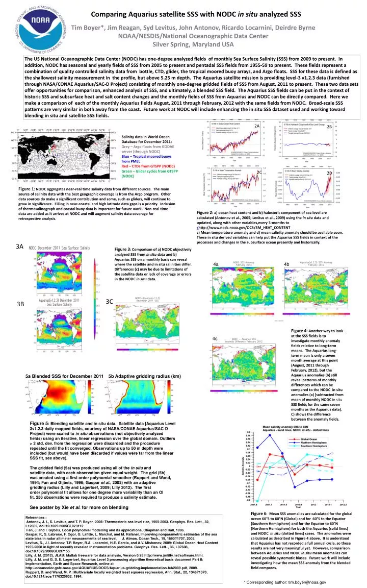
1. Comparing Aquarius satellite SSS with NODC in situ analyzed SSS Tim Boyer*, Jim Reagan, SydLevitus, John Antonov, Ricardo Locarnini, Deirdre Byrne NOAA/NESDIS/National Oceanographic Data Center Silver Spring, Maryland USA The US National Oceanographic Data Center (NODC) has one-degree analyzed fields of monthly Sea Surface Salinity (SSS) from 2009 to present. In addition, NODC has seasonal and yearly fields of SSS from 2005 to present and pentadal SSS fields from 1955-59 to present. These fields represent a combination of quality controlled salinity data from bottle, CTD, glider, the tropical moored buoy arrays, and Argo floats. SSS for these data is defined as the shallowest salinity measurement in the profile, but above 5.25 m depth. The Aquarius satellite mission is providing level-3 v1.2.3 data (furnished through NASA/CONAE Aquarius/SAC-D Project) consisting of monthly one-degree gridded fields of SSS from August, 2011 to present. These two data sets offer opportunities for comparison, enhanced analysis of SSS, and ultimately, a blended SSS field. The Aquarius SSS fields can be put in the context of historic SSS and subsurface heat and salt content changes and the monthly fields of SSS from Aquarius and NODC can be directly compared. Here we make a comparison of each of the monthly Aquarius fields August, 2011 through February, 2012 with the same fields from NODC. Broad-scale SSS patterns are very similar in both away from the coast. Future work at NODC will include enhancing the in situ SSS dataset used and working toward blending in situ and satellite SSS fields. 2A Salinity data in World Ocean Database for December 2011: Grey – Argo floats from GODAE server (through NODC) Blue – Tropical moored buoys from PMEL Red – CTDs from GTSPP (NODC) Green – Glider cycles from GTSPP (NODC) 2B 2C 2D Figure 1: NODC aggregates near-real time salinity data from different sources. The main source of salinity data with the best geographic coverage is from the Argo program. Other data sources do make a significant contribution and some, such as gliders, will continue to grow in significance. Filling in near-coastal and high latitude data gaps is a priority. Inclusion of thermosalinograph and coastal buoy data is important for future work. Non-real time data are added as it arrives at NODC and will augment salinity data coverage for retrospective analysis. Figure 2: a) ocean heat content and b) halosteric component of sea level are calculated (Antonov et al., 2005; Levitus et al., 2009) using the in situ data and updated, along with other variables,every 3-months to /http://www.nodc.noaa.gov/OC5/3M_HEAT_CONTENT c) Mean temperature anomaly and d) mean salinity anomaly should be available soon. These in situ derived variables can help put the Aquarius SSS fields in context of the processes and changes in the subsurface ocean presently and historically. 3A Figure 3: Comparison of a) NODC objectively analyzed SSS from in situ data and b) Aquarius SSS on a monthly basis can reveal where the satellite and in situ salinities differ. Differences (c) may be due to limitations of the satellite data or lack of coverage or errors in the NODC in situ data. 4a 4b 3C 3B 4c Figure 4: Another way to look at the SSS fields is to investigate monthly anomaly fields relative to long-term means. The Aquarius long-term mean is only a seven month average at this point (August, 2011 through February, 2012), but the Aquarius anomalies (b) still reveal patterns of monthly differences which can be compared to the NODC in situ anomalies (a) [subtracted from mean of monthly NODC in situ SSS fields for the same seven months as the Aquarius data]. C) shows the difference between the anomaly fields. 5a Blended SSS for December 2011 5b Adaptive gridding radius (km) Figure 5: Blending satellite and in situ data. Satellite data [Aquarius Level 3v1.2.3 daily mapped fields, courtesy of NASA/CONAE Aquarius/SAC-D Project) were scaled to in situ observations (not objectively analyzed fields) using an iterative, linear regression over the global domain. Outliers > 2 std. dev. from the regression were discarded and the procedure repeated until the fit converged. Observations up to 50 m depth were included (but would have been discarded if values were far from the linear SSS fit, see above). The gridded field (5a) was produced using all of the in situ and satellite data, with each observation given equal weight. The grid (5b) was created using a first order polynomial smoother (Ruppert and Wand, 1994; Fan and Gijbels, 1996; Gaspar et al., 2002) with an adaptive gridding radius (Lilly and Lagerloef, 2009; Lilly 2012). The first order polynomial fit allows for one degree more variability than an OI fit. 256 observations were required to produce a salinity estimate. See poster by Xie et al. for more on blending References:: Antonov, J. I., S. Levitus, and T. P. Boyer, 2005: Thermosteric sea level rise, 1955-2003. Geophys. Res. Lett., 32, L12602, doi:10.1029/2005GL023112 Fan, J. and I. Gijbels, Local polynomial modelling and its applications, Chapman and Hall, 1996. Gaspar, P., S. Labroue, F. Ogor, G. Lafitte, L. Marchal, and M. Rafanel, Improving nonparametric estimates of the sea state bias in radar altimeter measurements of sea level, J. Atmos. Ocean Tech., 19, 1690?1707, 2002. Levitus, S., J.I. Antonov, T.P. Boyer, R.A. Locarnini, H.E. Garcia, and A.V. Mishonov, 2009: Global Ocean Heat Content 1955-2008 in light of recently revealed instrumentation problems. Geophys. Res. Lett. , 36, L07608, doi:10.1029/2008GL037155 Lilly, J. M. (2012), JLAB: Matlab freeware for data analysis, Version 0.93,http://www.jmlilly.net/software.html. Lilly, J. M. and G. S. E. Lagerloef, Aquarius Level 3 processing algorithm theoretical basis document Part II: Implementation, Earth and Space Research, online at http://oceancolor.gsfc.nasa.gov/AQUARIUS/DOCS/Aquarius-gridding-implementation.feb2009.pdf, 2009. Ruppert, D. and Wand, M. P.: Multivariate locally weighted least squares regression, Ann. Stat., 22, 1346?1370, doi:10.1214/aos/1176325632, 1994. Figure 6: Mean SSS anomalies are calculated for the global ocean 60°S to 60°N (Global) and for 60°S to the Equator (Southern Hemisphere) and for the Equator to 60°N (Northern Hemisphere) for both the Aquarius (solid lines) and NODC in situ (dotted lines) cases. The anomalies were calculated as described in Figure 4 above. It is understood that Aquarius has not recorded a full annual cycle, so these results are not very meaningful yet.However, comparison between Aquarius and NODC in situ mean anomalies can reveal possible systematic biases. Future work will include investigating how the mean SSS anomaly from the blended field compares. * Corresponding author: tim.boyer@noaa.gov