Download
1 / 65
650 likes | 725 Views
Part III The General Linear Model Chapter 9 Regression. GLM, applied to regression. Example 9.3.1 from Snedecor and Cochran (1989 ) Interested in the relationship between: phosphorus content of corn ( Pcorn in ppm) & phosphorus levels in soil samples ( Psoil in ppm). 1. Construct Model.

E N D
GLM, applied to regression • Example 9.3.1 from Snedecorand Cochran (1989) • Interested in the relationship between: • phosphorus content of corn (Pcorn in ppm) & phosphorus levels in soil samples (Psoil in ppm).
1. Construct Model Verbal Formal Graphical
Graphical 1. Construct Model Verbal Phosphorus content of corn (Pcorn) depends on Phosphorus content of soil (Psoil)
1. Construct Model Phosphorus content of corn (Pcorn) depends on Phosphorus content of soil (Psoil) Verbal Formal Graphical
2. Execute analysis. Place data in model format: lm1 <- lm(Pcorn~Psoil, data=corn) 2. Execute analysis. Compute fitted values and residuals. fits <- fitted(lm1) resid <- residuals(lm1) cbind(corn, fits, resid)
3. Evaluate Model. Plot residuals against fitted values Check linear trend
3. Evaluate Model. Plot residuals against fitted values plot(fits,resid,pch=16) Check linear trend
3. Evaluate Model. • Using theoretical distributions (χ2, t, F) to calculate p-value, therefore we need to check their assumptions: • Fixed variance (errors homogeneous) • Normally distributed errors. • Independent errors • Unbiased estimate (errors sum to zero)
3. Evaluate Model. Independent errors. This is a text example, we do not have information on spatial layout of samples, or on collection sequence. We will assume independence 3. Evaluate Model. Conclusion. Residuals appear to homogeneous, but not normal. We assume independence, we do not have enough information to evaluate this assumption. We may need to use an empirical distribution to compute p-values or confidence limits
4. State population and whether sample is representative. Population? Sample (n=9) The population is all values of phosphorus in corn, given knowledge of phosphorus in the soil The sample is representative if the 17 soil types represent the range of possible soil types
5. Decide on mode of inference. Is hypothesis testing appropriate? • Since the relationship between P and P content in corn is unknown, we proceed 6. State HA / Ho, test statistic and α HA: Ho: Statistic: α:
7. ANOVA: partition df according to model. n=9 dftot = ________ = _____ dfmodel= 1 dfres= dftotal– dfmodel = _____
7. ANOVA: Calculate SS, partition according to model. Null model: Pcorn = mean(Pcorn) SS total: 2274.00 Regression model: 61.58 + 1.417*Psoil SS residual: 800.43 SS improvement? __________
7. ANOVA: Partition df, SS according to model. Complete ANOVA table 7. ANOVA: Calculate Type I error from F distribution. Packages compute and place the p-value in the ANOVA table p = 0.00885
8. Recompute p-value if necessary. • p-values can be inaccurate if assumptions are violated • Distortion depends on sample size • As a rule of thumb, distortion is greatest if n < 30 • less serious if 30 < n < 100 • usually not serious if n > 100 • When assumptions are not met, recompute Type I error if two conditions are met: • n small • p near α
8. Recompute p-value if necessary. • Due diligence recompute p-value using randomization • Free of assumptions • In 4000 randomizations there were 27 instances of an F-ratio greater than 12.89 • Empirical p-value: 0.00675 • Theoretical p-value: 0.008854
9. Declare and report decision about model terms. • p = 0.006750 (via randomization, hence no assumptions) • p < α= 5% so reject Ho for HA • Report decision with evidence: • There was a significant increase in available phosphorus with increase in soil phosphorus (F1,7 = 12.89, p = 0.00675 by randomization)
10. Report and interpret parameters of biological interest. • Regression Equation:
Today: Lab 4 due • Monday & Tuesday: No classes • Wednesday: Grad seminar Lecture Quizz5 • Thursday: Lab 5a
Chapter 9.2 Regression. Explanatory Variable Fixed into Classes
GLM, applied to regressionX variable fixed into classes • Example: Galton’s Law • Quantity of interest is the stature (height) of sons in relation to stature (height) of their fathers. • Data collected by Francis Galton at end of the 19th century. • 1st application of regression
1. Construct Model Verbal Data Formal Graphical
1. Construct Model Verbal There is a positive relation between heights of sons and fathers Data Explanatory: _____________ Response: _____________ Model: __________________ Formal Graphical
1. Construct Model … … …
2. Execute analysis. Place data in model format: … … … lm1 <- lm(Hson~Hf, weights=Nfamily, data=Heights)
2. Execute analysis. Compute fitted values and residuals. coefficients(lm1) (Intercept) Hf 33.2855960 0.5225171 … … …
3. Evaluate Model • Straight line model ok? • Errors homogeneous? • Errors normal? • Errors independent?
4. State population and whether sample is representative. • Population is all possible measurements, given the measurement protocol, if we repeated the study thousands of times • We infer a population consisting of thousands of runs of the same experiment, using the same protocol
5. Decide on mode of inference. Is hypothesis testing appropriate? • Might expect a 1:1 ratio • Undertake hypothesis testing? • Use confidence limits 10. Report and interpret parameters of biological interest. • Compute confidence limits from standard error of the slope parameter summary(lm1)$coefficients Coefficients: EstimateStd. Error t value Pr(>|t|) (Intercept) 33.28560 1.64243 20.27 2.61e-12 *** Hf 0.52252 0.02424 21.55 1.06e-12 ***
10. Report and interpret parameters of biological interest. • Confidence limits do not include hypothesis of • Nor does it include (i.e. no relationship) • is tightly centered around a value of ~0.5 • Great! But why?
Chapter 9.3 Regression. Explanatory Variable Measured with Error
GLM, applied to regressionExplanatory Variable Measured with Error • Adds bias to regression parameter estimates • Example: • Relation between number of eggs and body size in cabezon fish (Box 14.12, Sokaland Rohlf1995) • What is the magnitude of the bias?
V 1. Construct Model D F G • Verbal • Does egg number Neggsdepend on body mass M? • Graphical • Formal • Response: Neggs • Explanatory: M units? dimensions? measurement scale?
2. Execute analysis. Place data in model format: lm1 <- lm(Neggs~M, data=data) Estimate parameters and compute fitted values and residuals • The package first estimates the parameters of the general linear model, and • Where:
2. Execute analysis. Place data in model format: lm1 <- lm(Neggs~M, data=data) Estimate parameters and compute fitted values and residuals
3. Evaluate Model • Structure? • Straight line model ok? • Errors homogeneous? • Errors normal? • Errors independent? Where is measurement error If are normal and independent will be < by a factor of -Reliability ratio unknown, but no worse than measurement resolution (1 hectogram)
3. Evaluate Model • Structure? • Straight line model ok? • Errors homogeneous? • Errors normal? • Errors independent?
3. Evaluate Model M Neggs Res Lag.Res 14 61 15.05 NA 17 37 -14.56 15.05 24 65 0.35 -14.56 25 69 2.48 0.35 27 54 -16.26 2.48 33 93 11.52 -16.26 34 87 3.65 11.52 37 89 0.04 3.65 40 100 5.43 0.04 41 90 -6.43 5.43 42 97 -1.30 -6.43 • Structure? • Straight line model ok? • Errors homogeneous? • Errors normal? • Errors independent?