Download
1 / 24
810 likes | 2.08k Views
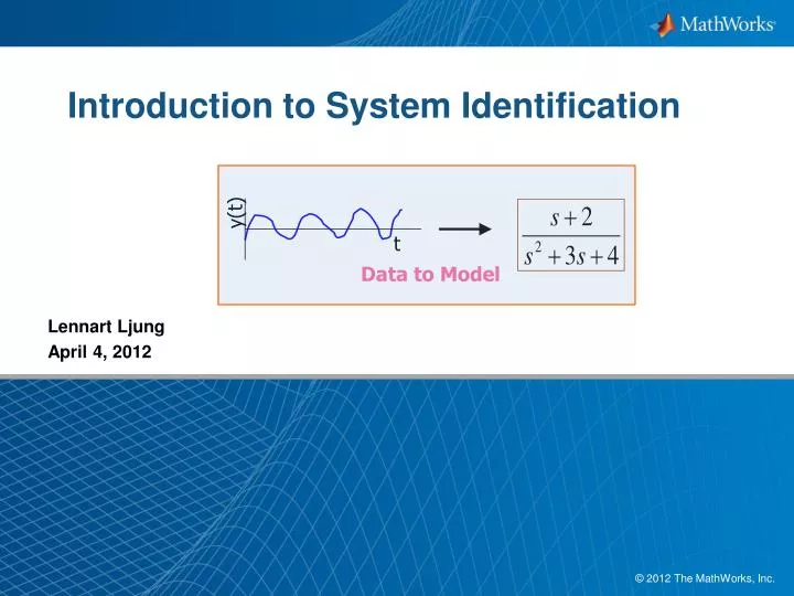
y(t). t. Data to Model. Introduction to System Identification. Lennart Ljung April 4 , 2012. Simscape SimMechanics SimHydraulics SimPowerSystems SimDriveline SimElectronics. Simulink Design Optimization. Neural Network Toolbox. Aerospace Blockset. Simulink.

E N D
y(t) t Data to Model Introduction to System Identification Lennart Ljung April 4, 2012
Simscape SimMechanics SimHydraulics SimPowerSystems SimDriveline SimElectronics Simulink Design Optimization Neural Network Toolbox Aerospace Blockset Simulink Modeling Dynamic Systems Modeling Approaches First-Principles Modeling Data-Driven Modeling System Identification Toolbox Tools for Modeling Dynamic Systems
The System Output Input velocity pitch angle rudders aileron thrust
The Model y u Output Input velocity pitch angle rudders aileron thrust u, y: measured time or frequency domain signals
The System and the Model System Measured input error + - Model Minimize
Fitting and Comparing Models • Core feature: Estimating models by tuning its parameters such that model outputs is close to measured output • COMPARE function: • Plots measured and model output curves together • Shows a numerical measure of fit: the percent of the output variation reproduced by the model DEMO: Model for data collected from a hair dryer Input signal: heating power Output signal: air temperature
Estimation and Validation Go Together • A large enough model can reproduce a measured output arbitrarily well. We must verify that model is relevant for other data – data that was not used for estimation, but was collected for the same system. Validation data Error DEMO: “Validate” the hair-dryer models on new data set Estimation data Number of parameters
Process of Building Models from Data • Gather experimental data • Estimate model from data • Select a structure • Find a model in it • Validate model with independent data
Model Structures in System Identification Tool (GUI) IDENT • Linear Parametric Models • Input-Output models (transfer functions) • State-space models • Linear Nonparametric models • Impulse response model IMPULSE, STEP • Frequency Response SPA, SPAFDR, ETFE • Process Models PEM • Nonlinear Models NLARX, NLHW
Transfer Functions and State Space Models • Linear models are typically described by state-space models IDSS (SSST) or transfer functions IDTF (TFEST) Transfer function B-order: nb (zeros) F-order: nf (poles) State-space Number of states: n • Both are just ways of writing a linear differential equation for relationship between input (u) and output (y) (take n=1)
Delays in TF and SS models • There could also be a delay (dead time) in the system: It takes nk samples before a change in u is visible in y. state space y nk transfer function u time • Linear parametric model structures are characterized by a few integers: n, or (npnz) and nk. • Commands such as n4sid, ssest, tfest use these integers to “create” models from data.
Handling Disturbance • Knowledge of nature of disturbance is useful: • Essential for predicting future system outputs, by understanding correlations between disturbances • Handling technique for identification: treat a disturbance source e as an extra unmeasured input. • e is not measured; its properties (white noise) are characterized statistically – mean, covariance state space transfer function e: disturbance source u system y input output DEMO: Models with disturbance component for hair-dryer data.
Non-Parametric Methods • Linear systems can also be described by non-parametric models that is curves that capture the system properties: • Transient responses • Frequency response • They can be estimated directly from data • Often useful to take a first look at these before parametric model estimation to get a feel for system’s basic properties.
Transient Response • A system’s transient response is its output to a transient like an impulse or step in its input. • Can be found by special experimentation with such inputs • For an existing model, its transient response is obtained by simulation with such inputs. IMPULSE, SIM, STEP • Estimation: From experimental input/output data, transient response is typically estimated via a flexible (high order) linear model. system u y
Frequency Response system • A system’s frequency response H(ω) is its response to a sinusoidal input sin(ωt). The output has same frequency ω but a different amplitude and a phase shift y(t) = A(ω) sin(ωt+ϕ(ω)) • Plotting A(ω) and ϕ(ω) vs. ω gives Bode plot. • Can be found experimentally by subjecting the system to sinusoidal inputs of various frequencies. • For an existing model, it is obtained from the z- or Laplace transform of the transfer function using z = exp(jωTs) or s = jω. • Estimation: From experimental input-output data, it may be estimated directly by using various Fourier-transform inspired techniques. SPA, SPAFDR, ETFE u y DEMO: Direct frequency and transient response estimation for dryer data
Process Models • Use a combination of gain (K), delay (Td) and one or more time constants (T) to describe the model. • Such forms are popular in process industry, hence called “process models”. IDPROC • Can be expanded to contain more poles, zeros and integrators. • Structure choices: • number/nature of poles • whether a delay element, a zero and/or an integrator should be included.
Use of Disturbance Model for Simulation and Prediction • Measured outputs contain disturbances. If there is a correlation between disturbances it is possible to better predict the future outputs from observing the past ones. DEMO: Models with disturbance component for hair-dryer data.
Residual Analysis Residuals = ”Leftovers” = 1-step-ahead predictionerrors error input e(t) Should be uncorr- elated with known things System t + - Whiteness Test Independence Test Model Check correlationfunctions! acceptable DEMO: Residual analysis on hair-dryer models
Putting the Model to Work • Use them for understanding a system’s behavior, and predicting future response of a system • Import estimated models into Simulink using dedicated blocks for simulation and code generation • Controller design: Import into SISOTOOL and MPC design task
y u Data Model Simplifying Complex Systems • Simplify complex Simulink model using simulation data. • Use Identified model to describe a component of a larger system
System Identification Toolbox Noise Model N • Control System Toolbox • Simulink Control Design • Robust Control Toolbox • Model Predictive Control Toolbox Controller Using Models for Control System Design Current Position • Estimate plant with parameter uncertainties • Estimate noise model Position Error Control Dynamic Model P + ∆P
More Information • Product page on mathworks.com: http://www.mathworks.com/products/sysid/ • Reach demos, webinars and documentation from here • Tech Support: http://www.mathworks.com/support/ • Textbooks • System Identification – Theory for the User, Lennart Ljung • System Identification – A frequency domain approach, RikPintelon, Johan Schoukens • Others…
Residual Analysis • Technique for validating a model’s quality. • Works by analyzing the residues which are differences between model’s response and measured values: where is the model’s best prediction of y(t) made at time t-1. • ε(t) should ideally be uncorrelated with information known at time t-1. Hence we test correlation between ε(t1) and u(t2) and also between ε(t1) and ε(t2), t1≠ t2