Download
1 / 30
360 likes | 647 Views
Regression and the Bias-Variance Decomposition. William Cohen 10-601 April 2008. Readings: Bishop 3.1,3.2. Regression. Technically: learning a function f( x )=y where y is real-valued , rather than discrete .

E N D
Regression and the Bias-Variance Decomposition William Cohen 10-601 April 2008 Readings: Bishop 3.1,3.2
Regression • Technically: learning a function f(x)=y where y is real-valued, rather than discrete. • Replace livesInSquirrelHill(x1,x2,…,xn) with averageCommuteDistanceInMiles(x1,x2,…,xn) • Replace userLikesMovie(u,m) with usersRatingForMovie(u,m) • …
Example: univariate linear regression • Example: predict age from number of publications
Linear regression • Model: yi = axi + b + εi where εi ~ N(0,σ) • Training Data: (x1,y1),….(xn,yn) • Goal: estimate a,b with w=(a,b) ^ ^ assume MLE
Linear regression • Model: yi = axi + b + εi where εi ~ N(0,σ) • Training Data: (x1,y1),….(xn,yn) • Goal: estimate a,b with w=(a,b) • Ways to estimate parameters • Find derivative wrt parameters a,b • Set to zero and solve • Or use gradient ascent to solve • Or …. ^ ^
Linear regression y2 d3 How to estimate the slope? d2 y1 d1 x1 x2 n*cov(X,Y) n*var(X)
Linear regression y2 d3 How to estimate the intercept? d2 y1 d1 x1 x2
Bias – Variance decomposition of error • Return to the simple regression problem f:XY y = f(x) + What is the expectederror for a learned h? noise N(0,) deterministic
Bias – Variance decomposition of error learned from D dataset true fct Experiment (the error of which I’d like to predict): 1. Draw size n sample D=(x1,y1),….(xn,yn) 2. Train linear function hD using D 3. Draw a test example (x,f(x)+ε) 4. Measure squared error of hD on that example
Bias – Variance decomposition of error (2) learned from D dataset true fct Fix x, then do this experiment: 1. Draw size n sample D=(x1,y1),….(xn,yn) 2. Train linear function hD using D 3. Draw the test example (x,f(x)+ε) 4. Measure squared error of hD on that example
Bias – Variance decomposition of error t ^ f ^ really yD y why not?
Bias – Variance decomposition of error Depends on how well learner approximates f Intrinsic noise
Bias – Variance decomposition of error VARIANCE Squared difference between best possible prediction for x, f(x), and our “long-term” expectation for what the learner will do if we averaged over many datasets D, ED[hD(x)] Squared difference btwn our long-term expectation for the learners performance, ED[hD(x)], and what we expect in a representative run on a dataset D (hat y) BIAS2
Bias-variance decomposition Make the long-term average better approximate the true function f(x) Make the learner less sensitive to variations in the data How can you reduce bias of a learner? How can you reduce variance of a learner?
A generalization of bias-variance decomposition to other loss functions • “Arbitrary” real-valued loss L(t,y) But L(y,y’)=L(y’,y), L(y,y)=0, and L(y,y’)!=0 if y!=y’ • Define “optimal prediction”: y* = argmin y’ L(t,y’) • Define “main prediction of learner” ym=ym,D = argmin y’ ED{L(t,y’)} • Define “bias of learner”: B(x)=L(y*,ym) • Define “variance of learner” V(x)=ED[L(ym,y)] • Define “noise for x”: N(x) = Et[L(t,y*)] Claim: ED,t[L(t,y) ] = c1N(x)+B(x)+c2V(x) where c1=PrD[y=y*] - 1 c2=1 if ym=y*, -1 else m=n=|D|
Example: univariate linear regression • Example: predict age from number of publications Paul Erdős Hungarian mathematician, 1913-1996 x ~ 1500 age about 240
Linear regression Summary: y2 d3 d2 y1 d1 • To simplify: • assume zero-centered data, as we did for PCA • let x=(x1,…,xn) and y =(y1,…,yn) • then… x1 x2
Onward: multivariate linear regression col is feature Multivariate Univariate row is example
regularized Onward: multivariate linear regression ^
regularized Onward: multivariate linear regression ^ What does increasing λ do?
regularized Onward: multivariate linear regression ^ w=(w1,w2) What does fixing w2=0 do (if λ=0)?
Growing tree: Split to optimize information gain At each leaf node Predict the majority class Pruning tree: Prune to reduce error on holdout Prediction: Trace path to a leaf and predict associated majority class [Quinlan’s M5] Regression trees - summary build a linear model, then greedily remove features estimated error on training data estimates are adjusted by (n+k)/(n-k):n=#cases, k=#features using to a linear interpolation of every prediction made by every node on the path
Regression trees – example 2 What does pruning do to bias and variance?
Kernel regression • aka locally weighted regression, locally linear regression, LOESS, …
Kernel regression • aka locally weighted regression, locally linear regression, … • Close approximation to kernel regression: • Pick a few values z1,…,zkup front • Preprocess: for each example (x,y), replace x with x=<K(x,z1),…,K(x,zk)> where K(x,z) = exp( -(x-z)2 / 2σ2 ) • Use multivariate regression on x,y pairs
Kernel regression • aka locally weighted regression, locally linear regression, LOESS, … What does making the kernel wider do to bias and variance?
Additional readings • P. Domingos, A Unified Bias-Variance Decomposition and its Applications. Proceedings of the Seventeenth International Conference on Machine Learning (pp. 231-238), 2000. Stanford, CA: Morgan Kaufmann. • J. R. Quinlan, Learning with Continuous Classes, 5th Australian Joint Conference on Artificial Intelligence, 1992. • Y. Wang & I. Witten, Inducing model trees for continuous classes, 9th European Conference on Machine Learning, 1997 • D. A. Cohn, Z. Ghahramani, & M. Jordan, Active Learning with Statistical Models, JAIR, 1996.