Download
1 / 43
430 likes | 925 Views
Lectures on Modeling and Data Assimilation Richard B. Rood NASA/Goddard Space Flight System Visiting Scientist, Lawrence Livermore National Laboratory May 7 - 13, 2005 Banff, Alberta, CANADA Plan of Presentations Models and Modeling Data Assimilation What is it? Why?

E N D
Lectures on Modeling and Data Assimilation Richard B. Rood NASA/Goddard Space Flight System Visiting Scientist, Lawrence Livermore National Laboratory May 7 - 13, 2005 Banff, Alberta, CANADA Banff, May 2005
Plan of Presentations • Models and Modeling • Data Assimilation • What is it? • Why? • Things to Think About • Coupled Modeling Banff, May 2005
Model and Modeling • Model • A work or construction used in testing or perfecting a final product. • A schematic description of a system, theory, or phenomenon that accounts for its known or inferred properties and may be used for further studies of its characteristics. Types: Conceptual, Statistical, Physical, Mechanistic, … Banff, May 2005
Types of Models(see also, Chapter 17, Peixoto and Oort, 1992) • Conceptual or heuristic models which outline in the simplest terms the processes that describe the interrelation between different observed phenomena. These models are often intuitively or theoretically based. An example would be the tropical pipe model of Plumb [1996], which describes the transport of long-lived tracers in the stratosphere. • Statistical models which describe the behavior of the observations based on the observations themselves. That is the observations are described in terms of the mean, the variance, and the correlations of an existing set of observations. Johnson et al. [2000] discuss the use of statistical models in the prediction of tropical sea surface temperatures. • Physical models which describe the behavior of the observations based on first principle tenets of physics (chemistry, biology, etc.). In general, these principles are expressed as mathematical equations, and these equations are solved using discrete numerical methods. Good introductions to modeling include Trenberth [1992], Jacobson [1998], Randall [2000]. Banff, May 2005
Conceptual/Heuristic Model • Observed characteristic behavior • Theoretical constructs • “Conservation” • Spatial Average or Scaling • Temporal Average or Scaling • Yields • Relationship between parameters if observations and theory are correct Plumb, R. A. J. Meteor. Soc. Japan, 80, 2002 Banff, May 2005
Big models contain little models Atmosphere atmos Thermosphere Mesosphere Stratosphere land ice Troposphere coupler Troposphere ocean Dynamics / Physics Advection Mixing Radiation Convection PBL Clouds Management of complexity But, complex and costly Where’s chemistry and aerosols?
What are models used for? • Diagnostic: The model is used to test the processes that are thought to describe the observations. • Are processes adequately described? • Prognostic: The model is used to make a prediction. • Deterministic • Probabilistic Banff, May 2005
What’s a mechanistic model? Mechanistic models have one or more parameters prescribed, for instance by observations, and then the system evolves relative to the prescribed parameters. Thermosphere Sink of energy from below Mesosphere Relaxation to mean state Stratosphere Stratosphere Troposphere Geopotential @ 100 hPa A mechanistic model to study stratosphere Banff, May 2005
Boundary Conditions Emissions, SST, … e Representative Equations DA/Dt = P –LA – n/HA+q/H e Discrete/Parameterize (An+Dt – An)/Dt = … (ed, ep) Theory/Constraints ∂ug/∂z = -(∂T/∂y)R/(Hf0) Scale Analysis Primary Products (i.e. A) T, u, v, F, H2O, O3 … (eb, ev) Derived Products (F(A)) Pot. Vorticity, v*, w*, … Consistent Simulation Environment(General Circulation Model, “Forecast”) (eb, ev) = (bias error, variability error) Derived Products likely to be physically consistent, but to have significant errors. i.e. The theory-based constraints are met. Banff, May 2005
Representative Equations • ∂A/∂t = – UA + M + P – LA – n/HA+q/H • A is some constituent • U is velocity “resolved” transport, “advection” • M is “Mixing” “unresolved” transport, parameterization • P is production • L is loss • n is “deposition velocity” • q is emission • H is representative length scale for n and q • All terms are potentially important – answer is a “balance” Banff, May 2005
Discretization of Resolved Transport • ∂A/∂t = – UA (A,U) Grid Point (i,j) Choice of where to Represent Information Choice of technique to approximate operations in representative equations Rood (1987, Rev. Geophys.) Gridded Approach Orthogonal? Uniform area? Adaptive? Unstructured?
Discretization of Resolved Transport Grid Point (i,j+1) Grid Point (i+1,j+1) (A,U) (A,U) (A,U) (A,U) Grid Point (i,j) Grid Point (i+1,j) Banff, May 2005
Discretization of Resolved Transport Grid Point (i,j+1) Grid Point (i+1,j+1) (U) (U) (A) (U) (U) Grid Point (i,j) Grid Point (i+1,j) • Choice of where to • Represent Information • Impacts Physics • Conservation • Scale Analysis Limits • Stability
Discretization of Resolved Transport • ∂A/∂t = – UA Line Integral around discrete volume ∫ Banff, May 2005
“Finite-difference” vs. “finite-volume” • Finite-difference methods “discretize” the partial differential equations via Taylor series expansion – pay little or no attention to the underlying physics • Finite-volume methods can be used to “describe” directly the “physical conservation laws” for the control volumes or, equivalently, to solve the integral form of the equations using the following 3 integral theorems: • Divergence theorem: for the advection-transport process • Green’s theorem: for computing the pressure gradient forces • Stokes theorem: for computing the finite-volume mean vorticity using “circulation” around the volume (cell) Lin and Rood (1996 (MWR), 1997 (QJRMS)), Lin (1997 (QJRMS), 2004 (MWR)) Banff, May 2005
Importance of your decisions(Tape recorder in full Goddard GCM circa 2000) FINITE-VOLUME Slower ascent Faster mean vertical velocity FINITE-DIFFERENCE Faster ascent Slower mean vertical velocity S. Pawson, primary contact Banff, May 2005
Importance of your decisions(Precipitation in full GCM) Spectral Dynamics Community Atmosphere Model / “Eulerian” Finite Volume Dynamics Community Atmosphere Model / “Finite Volume” Precipitation in California (from P. Duffy) Banff, May 2005
Some conclusions about modeling • Physical approach versus a mathematical approach • Pay attention to the underlying physics – seek physical consistency • How does my comprehensive model relate to the heuristic models? • Quantitative analysis of models and observations is much more difficult than ‘building a new model.’ This is where progress will be made. • Avoid coffee table / landscape comparisons Banff, May 2005
The Dark Path of Data Assimilation • Basics of Assimilation • Assimilation in tracer transport • Ozone assimilation Banff, May 2005
Data Assimilation • Assimilation • To incorporate or absorb; for instance, into the mind or the prevailing culture (or, perhaps, a model) • Model-Data Assimilation • Assimilation is the objective melding of observed information with model-predicted information. Attributes: Rigorous Theory, Difficult to do well, Easy to do poorly, Controversial (“Best” estimate) Banff, May 2005
Model Data Boundary Conditions Emissions, SST, … e (OPfOT + R)x = Ao – OAf DA/Dt = P –LA – n/HA+q/H e Discrete/Error Modeling (An+Dt – An)/Dt = … e Constraints on Increments ∂ug/∂z = -(∂T/∂y)R/(Hf0) Scale Analysis (eb, ev) reduced Ai≡ T, u, v, F, H2O, O3 … (eb, ev) Inconsistent Pot. Vorticity, v*, w*, … Consistent Assimilation Environment O is the “observation” operator; Pf is forecast model error covariance R is the observation error covariance; x is the innovation Generally assimilate resolved, predicted variables. Future, assimilate or constrain parameterizations. (T, u, v, H2O, O3) Data appear as a forcing to the representative model equation Does the average of this added forcing equal zero?
What do these things mean? (OPfOT + R)x = Ao – OAf Sat Rad Sat Rad Bal Geo Sat Rad Sat Rad Bal Geo Sat Rad Space and Time Interpolation To Measured Quantity Sat Rad Bal Geo Sat Rad Bal Geo Sat Rad Sat Rad Ship Tem Sat Rad Ship Tem Sat Rad Ship Tem Sat Rad Bal Geo Satellite Balloon Ship Radiance Geopotential Temperature Model Forecast O – The Observation Operator Banff, May 2005
What do these things mean? (OPfOT + R)x = Ao – OAf Radius of Influence Correlation aligned with flow? Errors: Variance and Correlation Banff, May 2005
Figure 5: Schematic of Data Assimilation System Observation minus Forecast Data Stream 1 (Assimilation) Statistical Analysis Analysis & (Observation Minus Analysis) Error Covariance Quality Control Data Stream 2 (Monitoring) Model Forecast Forecast / Simulation Banff, May 2005
Ozone Data TOMS/SBUV POAM/MIPAS Ozone Data Sciamachy MLS Forecast & Observation Error Models Statistical Analysis Statistical Analysis Analysis Q.C. Winds Temperature Tracer Model Short-term Forecast (15 minutes) Long-term forecast What does an assimilation system look like?(Goddard Ozone Data Assimilation System) Obs - Forecast Analysis Increments HALOE Sondes “Analysis” BALANCE, BALANCE, BALANCE! Banff, May 2005
Why do we do assimilation? • Global synoptic maps (Primary (Constrained) Product) • Unobserved parameters (Primary - Derived Product) • Ageostrophic wind, constituents, vertical information, • Derived products • Vertical wind / Divergence, residual circulation, Diabatic and Radiative information, tropospheric ozone, … • Forecast initialization • Radiative correction for retrievals • “Background,” a priori profile, for retrievals • Alternative to traditional retrieval • Instrument/Data System monitoring • Instrument calibration • Observation quality control • Model evaluation / validation Banff, May 2005
ECMWF,ERA-40 Banff, May 2005
The transport application A ( space, time ) Chemistry Transport Model (CTM) ∂A/∂t = – UA + M + P – LA – n/HA+q/H Transport / Chemistry Advection Mixing Convection PBL Emissions J Rates React. Rate Solver Wet/Dry Input Fields “ONE WAY COUPLER” Winds, Temperature, … Convective Mass Flux, Water, Ice, … Turbulent Kinetic Energy … Diabatic Heating … Atmospheric “Model” History Tape
The Transport Application Residual Circulation Wave Transport Planetary Synoptic (u*,v*) (u,v) MIXING Banff, May 2005
PDFs of total ozone: observations & CTM GCM-driven DAS-driven • Means displaced • Spread too wide • Means displaced • Half-width ok Too much tropical-extratropical mixing in DAS Douglass, Schoeberl, Rood and Pawson (JGR, 2003)
UKMO UKMO DAO DAO GCM Kinematic Diabatic Kinematic Diabatic Kinematic Kinematic: considerable vertical and horizontal dispersion Diabatic: vertical dispersion reduced (smooth heating rates) Three-dimensional trajectory calculations UKMO UKMO DAO DAO GCM (50 days) GCM shows very little dispersion, regardless of method used Assimilated fields are excessively dispersive Schoeberl, Douglass, Zhu and Pawson (JGR, 2003)
Transport have we reached a wall? TRANSPORT with winds from assimilation D Residual Circulation • Derived quantities are not physically consistent • Dynamic – Radiative equilibrium is not present • Bias acts as forcing and generates spurious circulations • Data insertion generates “noise” that grows and propagates relation to bias • Temperature constraint too weak to define winds? • Wallace and Holton (1968) • Thickness measurements too thick? Wave Transport Planetary Synoptic D C (u*,v*) MIXING (u,v) Banff, May 2005
Major assimilation issue: Bias Primary Products Errors, (eb, ev) = (bias error, variability error), errors usually reduced. Derived Products and unobserved parameters likely to be physically Inconsistent, errors likely to increase relative to simulation. Why? Consider Ozone and Temperature: How are they related? O3 – T, Chemistry (P and L) – Seconds – hours – O3 – T, Transport (U) – Hours – Days – O3 – T, Diabatic forcing – Days – Months – O3 – T, Other constituents – Seconds – hours – days – If adjust O3 and T by observations to be “correct” and if that “correction” is biased, then there has to be a compenradion somewhere in the Representative Equation. Usually it appears as a bias in unobserved parameters and leads to “inconsistent” results. Budgets do NOT balance.
Ozone Assimilation • Why? (Rood, NATO ASI Review Paper, 2003) • Monitoring instrument behavior • Improving radiative calculation • Models • Retrievals • Tropospheric ozone? • … • What? • Impact of new data, what does it mean? Banff, May 2005
MIPAS Ozone assimilation • Comparison of an individual ozone sonde profile with three assimilations that use SBUV total column and stratospheric profiles from: • SBUV • SBUV and MIPAS • MIPAS • MIPAS assimilation captures vertical gradients in the lower stratosphere • Model + Data capture synoptic variability and spreads MIPAS information MIPAS data
Monitoring Data System EP TOMS Going Bad Adjustment To change in observing system Banff, May 2005
Summary (1) • Good representation of primary products, T, wind, ozone • Model-data bias, “noise” added at data insertion, data insertion as a source of gravity waves provides difficult challenges • Derived products are often “non-physical,” and examples of improving primary products degrades derived products • Pushing model errors into the derived products • Need to incorporate Theory/Constraints into assimilation more effectively Banff, May 2005
Summary (2) • Can we really do “climate” with assimilated data sets? • Don’t do trends • If I worked in data assimilation what would I propose? • Primary products: New data, Bias correction • Derived products/Use in “Climate” studies: Fundamental physics of model, model improvement • Error covariance modeling? Data assimilation technique? Banff, May 2005
Statistical Analysis Q.C. Quality Control: Interface to the Observations Satellite # 1 Self-comparison DATA GOOD BAD SUSPECT Comparison to “Expected” Satellite # 2 Self-comparison GOOD! Intercomparison Non-Satellite # 1 Self-comparison O “Expected Value” MODEL Forecast Memory of earlier observations MONITOR ASSIMILATE
What we’re really interested in! When Good Data Go Bad? • Good Data • Normal range of expectation • Spatial or temporal consistency • Bad data • Instrument malfunction … • Cloud in field of view … • Operator, data transmission error • The unknown unknown • New phenomenon • Model failure • New extreme of variability Banff, May 2005
Statistical Analysis Statistical Analysis Analysis Q.C. Winds Temperature Tracer Model Short-term Forecast (15 minutes) Long-term forecast Link to the adaptive observing Obs - Forecast What to Observe? What to Process? Data Anomalies Analysis Increments Features “Analysis” Banff, May 2005
Model - Data Assimilation • Objective, Automated Examination and Use of Observing System. • All types of observations … need to write an observation operator. • Requires Robust “Sampling” Observing System as a Foundation • There is no controversy of “sampling” versus “targeted” observations. They are each an important part of scientific investigation. • Powerful Technique for Certain Applications. • Provides Information that might be used in Adaptive Observing (or Data Processing). • From Quality Control Subsystem • From Forecast Subsystem Banff, May 2005