Download
1 / 42
420 likes | 655 Views
Traffic Engineering for ISP Networks. Jennifer Rexford Computer Science Department Princeton University http://www.cs.princeton.edu/~jrex. Outline. Overview of Internet routing IP addressing and forwarding Interdomain and intradomain routing Optimization: Tuning routing to the traffic

E N D
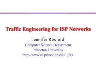
Traffic Engineering for ISP Networks Jennifer Rexford Computer Science Department Princeton University http://www.cs.princeton.edu/~jrex
Outline • Overview of Internet routing • IP addressing and forwarding • Interdomain and intradomain routing • Optimization: Tuning routing to the traffic • Optimizing routing given a topology and traffic matrix • Local search to select the integer link weights • Tomography: Inferring the traffic matrix • Estimating traffic matrix from routing and link loads • Conclusion and ongoing work
source destination IP network IP Service Model: Best-Effort Packet Delivery • Packet switching • Send data in packets • Header with source and destination address • Best-effort delivery • Packets may be lost • Packets may be corrupted • Packets may be delivered out of order
00001100 00100010 10011110 00000101 Packet Delivery Based on Destination IP Address • 32-bit number in dotted-quad notation (12.34.158.5) • Divided into network & host portions (left and right) • 12.34.158.0/24 is a 24-bit prefix with 28 addresses 12 34 158 5 Network (24 bits) Host (8 bits)
Longest-Prefix Match Forwarding • Forwarding tables in IP routers • Maps each IP prefix to next-hop link(s) • Destination-based forwarding • Packet has a destination address • Router identifies longest-matching prefix forwarding table 4.0.0.0/8 4.83.128.0/17 12.0.0.0/8 12.34.158.0/24 126.255.103.0/24 destination 12.34.158.5 outgoing link Serial0/0.1
Where do Forwarding Tables Come From? • Routers have forwarding tables • Map prefix to outgoing link(s) • Entries can be statically configured • E.g., “map 12.34.158.0/24 to Serial0/0.1” • But, this doesn’t adapt • To failures • To new equipment • To the need to balance load • That is where routing protocols come in…
Two-Tiered Internet Routing Architecture • Goal: distributed management of resources • Internetworking of multiple networks • Networks under separate administrative control • Solution: two-tiered routing architecture • Intradomain: inside a region of control • Okay for routers to share topology information • Routers configured to achieve a common goal • Interdomain: between regions of control • Not okay to share complete information • Networks may have different/conflicting goals
Autonomous Systems (ASes) • Autonomous Systems • Distinct regions of administrative control • Routers and links managed by an institution • Service provider, company, university, … • AS hierarchy • Tier-1 provider with national or global backbone • Regional provider with smaller backbone • Campus or corporate network • Interaction between ASes • Internal topology is not shared between ASes • … but, neighboring ASes interact to coordinate routing
AS Numbers (ASNs) Currently around 25,000 in use. • Level 3: 1 • MIT: 3 • Harvard: 11 • Yale: 29 • Princeton: 88 • AT&T: 7018, 6341, 5074, … • UUNET: 701, 702, 284, 12199, … • Sprint: 1239, 1240, 6211, 6242, … • … ASNs represent units of routing policy
Traffic Traverses Multiple ASes Path: 6, 5, 4, 3, 2, 1 4 3 5 2 6 7 1 Web server Client
Interdomain Routing: Border Gateway Protocol • ASes exchange info about who they can reach • IP prefix: block of destination IP addresses • AS path: sequence of ASes along the path • Policies configured by the AS’s network operator • Path selection: which of the paths to use? • Path export: which neighbors to tell? “I can reach 12.34.158.0/24 via AS 1” “I can reach 12.34.158.0/24” 2 3 1 data traffic data traffic 12.34.158.5
Interior Gateway Protocol (Within an AS) • Routers flood information to learn the topology • Routers determine “next hop” to reach other routers… • By computing shortest paths based on the link weights • Link weights configured by the network operator 2 1 3 1 3 2 1 5 12.34.158.0/24 Serial0/0.1 4 3
Constructing the Forwarding Table • Two routing protocols • BGP: learn the external route at some border router • IGP: learn outgoing link on path to other router • Router joins the data • Prefix 12.34.158.0/24 reached through red router • Red router reached via link Serial0/0.1 • Forwarding entry: 12.34.158.0/24 Serial0/0.1 • Router forwards packets • Lookup destination 12.34.158.5 in table • Forward packet out link Serial0/0.1
Topology information is flooded within the routing domain Best end-to-end paths are computed locally at each router. Best end-to-end paths determine next-hops. Based on minimizing some notion of distance Works only if policy is shared and uniform Examples: OSPF, IS-IS Each router knows little about network topology Only best next-hops are chosen by each router for each destination. Best end-to-end paths result from composition of all next-hop choices Does not require any notion of distance Does not require uniform policies at all routers Examples: RIP, BGP Two Kinds of Routing Protocols Link State Vectoring
Link Weights Control the Flow of Traffic • Routers compute paths • Shortest paths as sum of link weights • Operators set the link weights • To control where the traffic goes 2 1 3 1 3 2 3 1 5 4 3
Heuristics for Setting the Link Weights • Proportional to physical distance • Cross-country links have higher weights than local ones • Minimizes end-to-end propagation delay • Inversely proportional to link capacity • Smaller weights for higher-bandwidth links • Attracts more traffic to links with more capacity • Tuned based on the offered traffic • Network-wide optimization of weights based on traffic • Directly minimizes key metrics like max link utilization
Why Are the Link Weights Static? • Strawman alternative: load-sensitive routing • Link metrics based on traffic load • Flood dynamic metrics as they change • Adapt automatically to changes in offered load • Reasons why this is typically not done • Delay-based routing unsuccessful in the early days • Oscillation as routers adapt to out-of-date information • Most Internet transfers are very short-lived • Research and standards work continues… • … but operators have to do what they can today
Big Picture: Measure, Model, and Control Network-wide “what if” model Offered traffic Changes to the network Topology/ Configuration measure control Operational network
Traffic Engineering in an ISP Backbone • Topology • Connectivity and capacity of routers and links • Traffic matrix • Offered load between points in the network • Link weights • Configurable parameters for Interior Gateway Protocol • Performance objective • Balanced load, low latency, service level agreements … • Question: Given the topology and traffic matrix in an IP network, which link weights should be used?
Key Ingredients of Our Approach • Measurement • Topology: monitoring of the routing protocols • Traffic matrix: widely deployed traffic measurement • Network-wide models • Representations of topology and traffic • “What-if” models of shortest-path routing • Network optimization • Efficient algorithms to find good configurations • Operational experience to identify key constraints
Formalizing the Optimization Problem • Input: graph G(R,L) • R is the set of routers • L is the set of unidirectional links • cl is the capacity of link l • Input: traffic matrix • Mi,j is traffic load from router i to j • Output: setting of the link weights • wlis weight on unidirectional link l • Pi,j,lis fraction of traffic from i to j traversing link l
0.25 0.25 0.5 1.0 1.0 0.25 0.25 0.5 0.5 0.5 Multiple Shortest Paths With Even Splitting Values of Pi,j,l
f(x) x 1 Defining the Objective Function • Computing the link utilization • Link load:ul = Si,j Mi,j Pi,j,l • Utilization: ul/cl • Objective functions • min(maxl(ul/cl)) • minl(S f(ul/cl))
Complexity of the Optimization Problem • NP-hard optimization problem • No efficient algorithm to find the link weights • Even for the simple convex objective functions • Why can’t we just do multi-commodity flow? • E.g., solve the multi-commodity flow problem… • … and the link weights pop out as the dual • Because IP routers cannot split arbitrarily over ties • What are the implications? • Have to resort to searching through weight settings
Optimization Based on Local Search • Start with an initial setting of the link weights • E.g., same integer weight on every link • E.g., weights inversely proportional to link capacity • E.g., existing weights in the operational network • Compute the objective function • Compute the all-pairs shortest paths to get Pi,j,l • Apply the traffic matrix Mi,j to get link loads ul • Evaluate the objective function from the ul/cl • Generate a new setting of the link weights repeat
Making the Search Efficient • Avoid repeating the same weight setting • Keep track of past values of the weight setting • … or keep a small signature (e.g., a hash) of past values • Do not evaluate a weight setting if signatures match • Avoid computing the shortest paths from scratch • Explore weight settings that changes just one weight • Apply fast incremental shortest-path algorithms • Limit the number of unique values of link weights • Do not explore all 216 possible values for each weight • Stop early, before exploring the whole search space
Incorporating Operational Realities • Minimize number of changes to the network • Changing just 1 or 2 link weights is often enough • Tolerate failure of network equipment • Weights settings usually remain good after failure • … or can be fixed by changing one or two weights • Limit dependence on measurement accuracy • Good weights remain good, despite random noise • Limit frequency of changes to the weights • Joint optimization for day and night traffic matrices
Application to AT&T’s Backbone Network • Performance of the optimized weights • Search finds a good solution within a few minutes • Much better than link capacity or physical distance • Competitive with multi-commodity flow solution • How AT&T changes the link weights • Maintenance done every night from midnight to 6am • Predict effects of removing link(s) from the network • Reoptimize the link weights to avoid congestion • Configure new weights before disabling equipment
Example from My Visit to AT&T’s Operations Center • Amtrak repairing/moving part of the train track • Need to move some of the fiber optic cables • Or, heightened risk of the cables being cut • Amtrak notifies us of the time the work will be done • AT&T engineers model the effects • Determine which IP links go over the affected fiber • Pretend the network no longer has these links • Evaluate the new shortest paths and traffic flow • Identify whether link loads will be too high
Example Continued • If load will be too high • Reoptimize the weights on the remaining links • Schedule the time for the new weights to be configured • Roll back to the old weight setting after Amtrak is done • Same process applied to other cases • Assessing the network’s risk to possible failures • Planning for maintenance of existing equipment • Adapting the link weights to installation of new links • Adapting the link weights in response to traffic shifts
Conclusions on Traffic Engineering • IP networks do not adapt on their own • Routers compute shortest paths based on static weights • Service providers need to adapt the weights • Due to failures, congestion, or planned maintenance • Leads to an interesting optimization problems • Optimize link weights based on topology and traffic • Optimization problem is computationally difficult • Forces the use of efficient local-search techniques • Results of the local search are good • Near-optimal solutions that minimize disruptions
Ongoing Work • Robust link-weight assignments • Link/node failures • Range of traffic matrices • More complex routing models • Hot-potato routing • BGP routing policies • Interaction between ASes • Inter-AS negotiation for joint optimization • Grappling with scalability and trust issues
Computing the Traffic Matrix Mi,j • Hard to measure the traffic matrix • IP networks transmit data as individual packets • Routers do not keep traffic statistics, except link utilization on (say) a five-minute time scale • Need to infer the traffic matrix Mi,j from • Current topology G(R,L) • Current routing Pi,j,l • Current link load ul • Link capacity cl
Inference: Network Tomography From link counts to the traffic matrix Sources 5Mbps 3Mbps 4Mbps 4Mbps Destinations
Tomography: Formalizing the Problem • Ingress-egress pairs • p is a ingress-egress pair of nodes (i,j) • xp is the (unknown) traffic volume for this pair Mi,j • Routing • Plp is proportion of p’s traffic that traverses l • Links in the network • l is a unidirectional edge • ul is the observed traffic volume on this link • Relationship: u = Px (work backwards to get x)
Tomography: One Observation Not Enough • Linear system of n nodes is underdetermined • Number of links e is around O(n) • Number of ingress-egress pairs c is O(n2) • Dimension of solution sub-space at least c - e • Multiple observations are needed • k independent observations (over time) • Stochastic model with Poisson iid counts • Maximum likelihood estimation to infer matrix • Doesn’t work all that well in practice…
6 3 Approach Used at AT&T: Tomo-gravity • Gravitational assumption • Ingress point a has traffic via • Egress point b has traffic veb • Pair (a,b) has traffic proportional to via* veb 9 20 10
Approach Used at AT&T: Tomo-gravity • Problem with gravity model • Gravity model ignores the load on the inside links • Gravity assumption isn’t always 100% correct • Resulting traffic matrix might not satisfy the link loads • Combining the two techniques • Gravity: find a traffic matrix using the gravity model • Tomography: find the family of traffic matrices consistent with all link load statistics • Tomo-gravity: find the tomography solution that is closest to the output of the gravity model • Works extremely well (and fast) in practice
Conclusions • Managing IP networks is challenging • Routers don’t adapt on their own to congestion • Routers don’t reveal much information about traffic • Measurement provides a network-wide view • Topology • Traffic matrix • Optimization enables the network to adapt • Inferring the traffic matrix from the link loads • Optimizing the link weights based on the traffic matrix
New Research Direction: Design for Manage-ability • Two main parts of network management • Control: optimization • Measurement: tomography • Two research approaches • Bottom up: do the best with what you have • Top down: design systems that are easier to manage • Design for manage-ability • “If you are both the professor and the student, you create exam questions that are easy to answer.” – Mung Chiang