Download
1 / 52
530 likes | 1.13k Views
Forwards, Futures, and Swaps Payoff of d erivative security is tied to underlying security. Underlying security determines the price of the derivative security .

E N D
Forwards, Futures, and Swaps • Payoff of derivative security is tied to underlying security. • Underlying security determines the price of the derivative security. • Example. Forward contract to purchase 2,000 pounds of sugar at 12 cents per pound in 6 month. If the price of sugar then were 13 cents per pound, the contract would have a value of 1 cent per pound or $20 (owner can buy sugar and sell it on the market with profit). Chapter 10
Example.Option to purchase 100 shares of GM stock for $60 per share in 3 month. • Example. Home insurance. • Example.Swap = exchange of cash flows ( for instance, exchange of baskets of variable rate and fix rate mortgages). • Example. You are purchasing a fur coat which is free if the weather ... Chapter 10
Forward contracts • A forward contract on a commodity is a contract to purchase or sell a specific amount of the commodity at a specific price and at a specific time (for instance, the sugar contract which we have considered). • The contract is between two parties, the buyer and seller. The buyer has long position and seller has short position. • Usually initial payment is zero. • The forward price is the price that applies at delivery. Chapter 10
The open market for immediate delivery of underlying asset is called spot market . • Forward market trades contracts for future delivery. Forward interest rates • The forward interest rate was defined as the rate of interest associated with an agreement to loan money over a specified interval of time in the future • The forward rates may be defined from the term structure of the interest rates. They are basic to the pricing of forward contracts of all commodities. Chapter 10
Example 10.1 (A T-bill forward) You arrange to loan money for 6 month beginning 3 month from now. Suppose that yearly forward rate for that period in 10% (5% for 6 month). The price would be agreed upon today. The T-bill will pay at maturity $1,000. Hence the value of T-bill would be $1,000/1.05 = 952.38 (with 10% rate). The actual value of T-bill in 3 month may differ from 952.38, so you can get or loose money. Chapter 10
Forward prices • Forward price F = delivery price of a unit of the underlying asset to be delivered at a specific future date. • The forward price F is determined such that the current value f of the contract equals zero (i.e., f=0). The value of the contract may further evolve, but it starts from zero point. • We will derive the forward price F associated with contract written at time t=0 to deliver an asset at time T . Chapter 10
Assumptions: no transaction costs; it is possible to store the underlying asset without cost; it is possible to sell the underlying asset short. • Assumptions are reasonable for sugar or gold, but not good for perishables. • Let us show that the forward delivery price F of the underlying asset is determined by the spot and forward interest rates. • Suppose that at t=0 the underlying asset price is S. And forward contract is designed to deliver at time T. Chapter 10
The contract (for one unit) is equivalent to the cash flow stream (-S,F). You can buy at time t=0 on the market a unit of asset with price S, which is equivalent to the cash flow -S, and sell at time t=T with price F, which gives the cash flow F. PV (-S,F) = 0 => -S+d(0,T)F=0 => F= S/d(0,T) Chapter 10
Forward price formula : F= S/d(0,T) Proof. (1)Suppose that F > S/d(0,T) . Construct portfolio: borrow S at time t=0; buy on the market a unit of asset with price S; sell with price F at time T; repay the loan S/d(0,T); get profit F-S/d(0,T). This is an arbitrage. Table 10.1 (details of transactions) At Time t=0 Initial cost Final receipt Borrow $S -S - S/d(0,T) Buy 1 unit and store S 0 Short 1 forward 0 F . Total 0 F-S/d(0,T) Chapter 10
Proof (Cont’d) (2) Suppose that F < S/d(0,T) . Construct portfolio: sell short a unit of the asset and get S (borrow from somebody the asset, sell it on the market at t=0); invest in the bank S at t=0, receive S/d(0,T) at time T; repurchase the asset at time t=T and spend F, then return borrowed asset. Profit = S/d(0,T) - F (arbitrage). Table 10.2 (details of transactions) At Time t=0 Initial cost Final receipt Lend $S S S/d(0,T) Short 1 unit -S 0 Go long 1 forward 0 -F . Total 0 S/d(0,T)- F Chapter 10
Example 10.2 (Copper forward) A manufactures of electrical equipment wants to take the long side of a forward contract for delivery of copper in 9 month. The current price of copper in 84.85 cents per pound, 9-month T-bill is selling at 970.87. What is the price of the forward contract? If we ignore the cost of storing, the price equals 84.85*(1000/ 970.87)=87.4 per pound. Chapter 10
Forward price at time zero equals the projected future value of a cash of amount S(0) . F0 observed spot rate S0 projected spot rate T Chapter 10
Example 10.3 (Continuous time compounding) If there is a constant interest rate r compounded continuously, the forward rate formula becomes F = S erT • The discount rate d(0,T) used in the forward price formula should be consistent with market interest rate. Traders of forward and futures use so called repo rate associated with the repurchase agreement (it takes into account roundtrip sell and repurchase). Repo rate is slightly higher than T-bill rate. Chapter 10
Cost of Carry • The preceding analysis assumes that there are no storage costs. • We use a discrete-time (multi-period) model. The delivery date T is M periods in future. The carrying cost is c(k) per unit of holding the asset in the period from k to k+1. The initial spot price is S. The discount factor from k to M is denoted by d(k,M) . • The forward price of an asset is determined by the structure of the forward interest rates. Chapter 10
Forward price formula with carrying costs. Suppose that the asset can be sold short, then the theoretical forward price is F = S/d(0,M) + ∑c(k)/ d(k,M) . Equivalently S = - ∑d(0,k) c(k) + d(0,M) F . Idea of the proof: Present value of the cash flow stream ( -S-c(0), -c(1), -c(2),..., c(M-1), F ) must be zero. Chapter 10
Proof. (1)Suppose that F > S/d(0,M) +∑ c(k)/ d(k,M) We can construct an arbitrage. Table 10.3 (details of transactions) Time 0 action Time 0 cost Time k cost Receipt at time M Borrow $S -S 0 - S/d(0,M) Buy 1 unit spot S 0 0 Short 1 forward 0 0 F Borrow c(k)’s forward - c(0) - c(k) - ∑ c(k)/ d(k,M) Pay storage c(0) c(k) 0 . Total 0 0 F-S/d(0,M)-∑ c(k)/ d(k,M) Similar, with short-selling assumption we can prove F < S/d(0,M) +∑ c(k)/ d(k,M) is impossible. Chapter 10
Example 10.4. (Sugar with storage cost) The current price of sugar is 12 cents per pound. The carrying cost in 0.1 cents per pound per month (to be paid in the beginning of month). Interest rate is constant 9%. Price of sugar to be delivered in 5 month? Interest rate is 0.09/12=0.0075 per month. F=(1.0075)5(.12)+[ (1.0075)5+(1.0075)4 +(1.0075)3 +(1.0075)2+(1.0075)](0.001) =$ .1295=12.95 cents Chapter 10
Example 10.5 (A bond forward) Consider a treasury bond with a face value of $10,000, a coupon of 8%, and several years to maturity. Currently this bond is selling for $9,260, and the previous coupon has just been paid. Interest rate is flat for 1 year at 9%. What is the forward price of delivery of this bond in 1 year? Present value equation: S = ∑ d(0,k) c(k) + d(0,M) F . Using this equation $9,260=(F+$400)/(1.045)2+$400/1.045 => F= $9,294 . Chapter 10
Tight Markets The commodity theory suggests that the forward price will increase smoothly as the delivery date increases ( F = S/d(0,M) + ∑ c(k)/ d(k,M) ) . In practice this may not be the case !!! Table 10.4. Soybean Meal Forward Prices. Dec 188.2, Jan 185.6, Mar 184.0, May 183.7, Jul 184.8, Aug 185.50, Sep 186.2, Oct 188.0, Dec 189.0 Why farmers do not sell their holding and buy the forward contracts (sell Dec 188.2 and buy back Jul 184.8)? Soybean may be in short supply and it is convenient to have it on hand. Sell short also may not work: nobody will lend soybean meal. Chapter 10
Shorting relies on having excess stock over the entire period. If stock is low (or potentially may be low), short-selling at the spot price is infeasible. • Therefore, the theoretical relation holds in one direction as long as storage is possible F ≤ S/d(0,M) + ∑ c(k)/ d(k,M) • The inequality can be converted to equality by defining a convenience yield variable y F = S/d(0,M) + ∑ c(k)/ d(k,M) - ∑ y/ d(k,M) Chapter 10
The Value of a Forward Contract • A forward contract was written in the past with a delivery price F0 . At the present time t the forward price for the same delivery date is Ft . What is the current value ft of initial contract? The value of the forward: ft=(Ft - F0) d(t,T) Proof. Portfolio: one unit long of forward with delivery price Ft and one unit short with delivery price F0 . This is equivalent to cash flow F0 -Ft at time T . The present value of the portfolio is ft + (F0 -Ft ) d(t,T) , and this must be zero. Chapter 10
Swaps • Swap is an agreement to exchange one cash flow to another. • Plain vanilla swap is exchange of series of fixed level payments for a series of variable-level payments. • For instance, the plain vanilla interest rate swap is an exchange of a cash flow stream with fixed rate payments to a cash flow stream with variable rate payments. • Insurance is a swap. Chapter 10
Example. Commodity swap. Fixed payments Power company Swap counterparty Spot payments equivalents Real spot Oil payments Spot oil market Chapter 10
Value of a Commodity Swap • Party A receives spot price for N units of a commodity each period while paying a fixed amount X per unit for N units. For M periods, the net cash flow received by A is ( S1-X, S2-X, … , SM-X ) • Suppose that we are indifferent between receiving the Si (which is uncertain) and fixed Fi at time i . Discounting give the value of the stream V = ∑ d(0,i) (Fi-X) N The value of the swap can be determined from the series of forward prices. Chapter 10
Example 10.6 ( A gold swap ) Company receives spot value for gold in return for fixed payments. Assume that gold is in ample supply and can be stored without cost. In this case the forward price is Fi = S0 / d(0,i) . V = ∑ d(0,i) (Fi-X) N =[∑ d(0,i) Fi- ∑ d(0,i) X] N = [ ∑ S0- ∑ d(0,i) X] N = [ MS0- ∑ d(0,i) X] N The term ∑ d(0,i) X is a bond maturing at time M minus (misprint plus in the book) principal payment at maturity ∑ d(0,i) X = (X/C)[B(M,C)-100d(0,M)] where B(M,C) is the price (relative to 100) of a bond of maturity M and coupon C per year. Chapter 10
Example 10.6 ( Cont’d ) Indeed, suppose F=100=face value of the bond, C=coupon rate. M=number of periods B(M,C) = price of the bond Price of the bond equals B(M,C) = ∑ d(0,i) C + d(0,M) F Consequently, ∑ d(0,i) C = B(M,C) - d(0,M) F ∑ d(0,i) X = (X/C)[B(M,C)-100d(0,M)] Chapter 10
Value of an Interest Rate Swap. Consider a plain vanilla swap. Similar to the commodity swap we have cash flow stream (c0-r, c1-r, c2-r, … , cM-r) where r is the fixed rate and ci is the floating rate. The PV of cash flow stream with fixed rate equals r ∑ d(0,i) N Earlier we learn that the initial value of the floating rate bond is par: N - d(0,M) N . Hence the overall value of swap is V = [1- d(0,M) - r ∑ d(0,i) ]N . Chapter 10
Basics of Futures Contracts • Trading of forward contracts at the exchange is difficult to implement. - the delivery dates, quantities of delivered goods (per contract), delivery locations can be standardized; - forward prices is difficult to standardize (large number of forward prices). • Futures market is an alternative to the forward market. The futures contracts are revised each day. The process of revising (adjusting) is called marking to market. Chapter 10
Explanation of a futures contract • Suppose that at the first day a futures contract is written with the delivery price F0 . The price at the second day for the contract is F1 (e.g., F1- F0 >0 ) . At the second day, the clearing house associated with exchange revises all the contracts to the new price F1 . Long contract holders receive F1- F0 per unit of commodity, and short contract holders pay F1- F0 per unit of commodity (50% of investors are laughing and 50% are crying). • Actual deliveries under terms of futures contracts are quite rare (90% of all contracts are closed before delivery date). Chapter 10
Grains and Oilseeds Chapter 10
Margin account • Margin account is used to cover the futures price change. This account (usually) contains 5-10% of the value of the contract. The margin account is marked to market at the end of each day. • If the value of a margin account should drop below a defined maintenance margin level (usually about 75% of the initial margin requirement), a margin call is issued to the contract holder, demanding additional payments. Otherwise, the futures position will be closed out. Chapter 10
Example 10.7 (Margin) • Long position of one contract in corn (5,000 bushels, 1 bushel = 8 gallons) for March delivery at $2.10 (per bushel), margin=$800, maintenance margin=$600. • The next day the price of contract drops to $2.07. Loss=0.03* 5,000 =$150. The balance on margin account=800-150=$650. • The following day the price of contract drops to $2.05 and the loss=$100. The margin account is $550 which is below maintenance level $600. • The broker informs investor, that he/she must deposit $50 to the margin account otherwise his position will be closed (with account value $550). Chapter 10
Futures Prices • Only one price is associated with the price of futures contract- the delivery price. Contract value is always zero (marked to market). • As maturity day approaches the futures price and the spot price must approach each other; it is called convergence (see figure at the following page). • With forwards, there is no cash flows until the delivery date. With futures, there is cash flow each period. Chapter 10
Convergence of futures price and spot price Price Futures price Spot price T Chapter 10
Futures-forward equivalence Under assumption the interest rate are deterministic and follow the expectation dynamics, the forward and futures prices are identical. Proof. Initial futures price = F0 , initial forward price= G0 F0 F1 F2 FT=ST Let d(j,k) denote the discount rate at time j for a bond of unit face value maturing at time k . Chapter 10
Strategy A • At time 0: Go long d(1,T) futures. • At time 1: Increase position to d(2,T). . . . • At time k: Increase position to d(k+1,T). • At time T: Increase position to 1. Profit at time k + 1 from the previous period is (Fk+1- Fk) d(k+1,T) . We invest this profit at time k+1 in the interest rate market until time T. It is thereby transformed to the final amount [d(k+1,T)/d(k+1,T)](Fk+1 - Fk) = Fk+1- Fk => profitA= ∑ (Fk+1 - Fk) = FT - F0 = ST - F0 Chapter 10
Note that at each step before the end, the cash flow with strategy A equals zero because all profits are absorbed by the investing. Strategy B Take a long position in one forward contract. This requires no initial investment and produces a profit of profitB = ST - G0 . Chapter 10
We can now form a new strategy, which is A-B. This combined strategy also requires no cash flow until the final period, at which point it produces profit of G0 - F0. This is a deterministic amount, and hence must be zero if there is no opportunity for arbitrage. Hence G0 = F0.This statement finalizes the proof. • When the interest rate are not deterministic, the equivalence may not hold. However, this approach is used in hedging of futures with forward contracts (involving cash flows only at the delivery date). Chapter 10
Example 10.8. The company wants to buy 500,000 bushel of wheat forward for May delivery. Company uses futures for this purpose. The current futures (or forward) price for May delivery is $3.3 per bushel. The size of a standard contract is 5,000 bushels. The following table shows three possible scenarios: (1) using forward, profit equals 22 cents per bushel, total profit equals $110,000; (2) using futures, 100 contracts, total is $110,000 + interest; (3) futures strategy presented in the proof gives 109,952. Since interest is 1% per month, initially company goes 97 contracts long and then increases this by 1 contract per month.The forward contract is closely duplicated by the futures contract. Chapter 10
Futures and Forward Transactions, Table 10.5 Chapter 10
The Perfect Hedge • Perfect hedge = risk associated with a future commitment is completely eliminated by taking an equal and opposite position in the futures market. • Perfect hedgeis possible only if there is a future contract that matches your future commitment. Chapter 10
Example 10.9 (Wheat hedge, extension of Ex. 10.8) • The company needs to buy 500,000 bushel of wheat in May (spot market in May). The current futures (or forward) price for May delivery is $3.3 per bushel. • Hedging can be done by taking an equal and opposite (i.e., long, “buy now”) position in futures. • The net effect is that the producer will buy with the price $3.3 per bushel. Chapter 10
Example 10.10 ( A foreign currency hedge) • A company will receive 500,000 DM in 90 days. • The exchange risk (DM => $) can be hedged with four short (“sell now”) 125,000 DM contracts with 90 days maturity date. Chapter 10
The Minimum-Variance Hedge • It is not always possible to form a perfect hedge with futures contract (the delivery dates, the amount of assets, lack of liquidity). • The measure of the lack of the hedge is the basis, which is a mismatch between the spot and futures prices: basis = spot price of asset to be hedged - futures price of contract to be used Chapter 10
For instance, the obligation is to purchase W units of an asset at time T, where S is a spot price at time T. Cash flow related to purchasing equals x= WS. • Cash flow related to hedging equals (FT - F0)h, where F0 and FT arefutures prices and h is size of the contract. • Combined cash flow equals cash flow = y = x + (FT - F0)h • The variance of cash flow equals ( ^ denotes mean) var(y) = E[x-x^ + (FT - FT^)h]2 = var(x) + 2cov(x, FT)h+ var(FT) h2 (*) Chapter 10
Differentiating w.r.t. h of the variance and equating to zero gives var(y) = (var(x) + 2cov(x, FT)h+ var(FT) h2) = 2cov(x, FT) + 2 var(FT) h = 0 => h= - cov(x, FT) / var(FT) By substituting h value in (*) we get var(y) = var(x) - cov(x, FT)2 / var(FT) Minimum variance hedging formula h= - cov(x, FT) / var(FT) var(y) = var(x) - cov(x, FT)2 / var(FT) Chapter 10
When the obligation equal x= WST , minimal variance hedge equals h = - cov(x, FT) / var(FT) = - cov(WST, FT) / var(FT) = - W cov(ST, FT) / var(FT) = - βW , where β = cov(ST, FT) / var(FT) • This formula reminds the general CAPM formula for beta . Chapter 10
Example 10.11 (The perfect hedge) Suppose the FT=ST , i.e. we can make a perfect hedge h = - cov(x, FT) / var(FT) = - W cov(ST, FT) / var(FT) = - W cov(FT, FT) / var(FT) = - W var(FT) / var(FT) = - W Chapter 10
Example 10.12 (Hedging foreign currency with alternative futures) • A company will receive 1 million of Danish kroner in 60 days. • The exchange risk (Danish kroner => $) can not be perfectly hedged because of unavailability of Danish kroner futures. Hedging is done using DM. • Exchange rates: K=.165 $/kroner, M=.625 $/DM , K/M = .165/.625 = .262 DM/kroner . • The simplest idea is to sell short 262,000 DM which is equivalent to 1 million of kroners . Chapter 10
Data analysis shows that cor(K,M) = σMK/(σMσK)= 0.8; σM=3%; σK=2.5% . • We define x= K*million , FT = $ value of DM at time T, ST = K at time T . Minimum variance hedging formula: h = - β W , β = cov(ST, FT) / var(FT) = cov(K,M)/var(M) = σMK /(σM)2 = (σMK / (σMσK))*(σK /σM) = 0.8*(0.025K/0.03M) h = - β million = - 0.8*(0.025/ 0.03)* 0.262 million = -175,000 DM Chapter 10