Download
1 / 33
350 likes | 892 Views
PHASE CHANGES OF WATER Gibbs phase rule Thermodynamic surface for water Unusual properties of water. Gibbs Phase Rule For a closed, homogeneous system of constant composition (e.g., an ideal gas), we require two

E N D
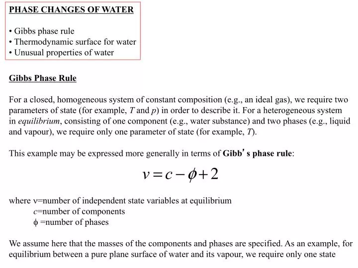
PHASE CHANGES OF WATER • Gibbs phase rule • Thermodynamic surface for water • Unusual properties of water Gibbs Phase Rule For a closed, homogeneous system of constant composition (e.g., an ideal gas), we require two parameters of state (for example, T and p) in order to describe it. For a heterogeneous system in equilibrium, consisting of one component (e.g., water substance) and two phases (e.g., liquid and vapour), we require only one parameter of state (for example, T). This example may be expressed more generally in terms of Gibb’s phase rule: where =number of independent state variables at equilibrium c=number of components =number of phases We assume here that the masses of the components and phases are specified. As an example, for equilibrium between a pure plane surface of water and its vapour, we require only one state
state variable, T, say. The equilibrium vapour pressure is a function of T, i.e., es=es(T). Thermodynamic Surface for Water The thermodynamic surface for water is shown in the diagram below (from Iribarne and Godson, “Atmospheric Thermodynamics”, page 60):
A projection of this surface onto the p-T plane is shown in the accompanying diagram: Note the supercooled water-vapour equilibrium which is not shown on the 3D thermodynamic surface. The following data, relating to this phase diagram, may be useful: LATENT HEATS lv=2.501106 Jkg-1 Note that ls=lv+lf and that the latent heats are functions of lf=0.334106 Jkg-1 temperature (Kirchoff’s law). (v=vapourization, f=fusion, ls=2.835106 Jkg-1 s=sublimation)
TRIPLE POINT This is the point at which all three phases of water substance co-exist in equilibrium. There are no independent (variable) parameters of state. The state variables are all specified (hence the term “point”), as given below. pt=0.6107 kPa (~35 km up in the atmosphere) Tt=273.16 K vs,t=1.09110-3 m3 kg-1 vl,t=1.00010-3 m3 kg-1 vv,t=206 m3 kg-1 Note: the specific volume of ice is larger than the specific volume of liquid water! CRITICAL POINT This is the point at which the distinction between liquid and vapour (the meniscus) disappears: pc=218.8 atm Tc=647 K vc=3.0710-3 m3 kg-1 UNUSUAL PROPERTIES OF WATER: Maximum density at 4oC: Water has its maximum density at 4oC rather than at the freezing point as is the case for most other liquids. Cooling below this point causes the density to decrease rather than increase. The explanation of this phenomenon has to do with the competing effects
which occur just above freezing. First, the density tends to increase as the temperature drops because of the reduction in thermal agitation of the molecules. However, as one approaches the freezing point, ice-like molecular clusters begin to form in the liquid. These have a lower density because of the less compact molecular packing in the crystal structure of ice (remember…ice floats!). Far from the freezing point, the first effect predominates. As the temperature approaches the freezing point, the second effect becomes dominant and the density decreases. The consequence of this property of water is that deep bodies of fresh water must cool to 4oC before their surface can cool towards the freezing point. Further cooling leads to ice formation on top of the liquid rather than at the bottom (which is what would occur if the maximum density occurred at the freezing point). This has enormous implications for the survival of fish, amphibians, and plant life over the winter. It also has implications for skating on natural ice! 2. Solid form is less dense than liquid form This is a most unusual property, some of whose consequences are icebergs, jökulhlaups (glacial outburst floods: images ), arctic pack ice, and the unusual way in which graupel and small hail melt. Ice is also unusual as a solid since most environmental ice exists at a high homologous temperature (this is the ratio of the actual temperature to the melting point temperature). Most other natural solids exist well below their melting point.
3. Greatest Specific Heat among Liquids Water: 4.2103 Jkg-1 K-1 Ethyl alcohol: 2.5103 Jkg-1 K-1 Mercury: 1.3102 Jkg-1 K-1 Because of its high specific heat capacity, bodies of water are good heat reservoirs. Our world’s oceans have a moderating effect on climate. 4. Greatest Latent Heat of Vapourization amongst Liquids Water: 2.5106 Jkg-1 Ethyl alcohol: 0.86106 Jkg-1 Mercury: 0.3106 Jkg-1 The latent heat of condensation plays a very important role in cloud and storm formation and drives much of the dynamics of the atmosphere. 5. Greatest Thermal Conductivity of all Liquids (except liquid metals) Water: 5.9510-5 Wm-1K-1 Ethyl alcohol: 1.7810-5 Wm-1K-1 Mercury: 810-4 Wm-1K-1 Water isn’t a particularly good insulator (you get cold while swimming!) Hence wet clothes or
wet insulation in your house provide poor protection from the cold. 6. Greatest Dielectric Constant of (almost) all Substances Hydrocyanic acid: 10210-11 Fm-1 Water: 7110-11 Fm-1 Ethyl Alcohol: 2210-11 Fm-1 Glass: 610-11 Fm-1 Ebonite: 210-11 Fm-1 Ice: 210-11 Fm-1 Air: 0.910-11 Fm-1 The dielectric constant, , enters Coulomb’s law in the denominator: The higher the dielectric constant the smaller the force between two oppositely charged ions in solution, so dissolved salts tend to stay dissolved in water. The result is that water is almost a universal solvent, a rather important result for atmospheric and oceanic chemistry. 7. Greatest Surface Tension of any Liquid except Mercury Water: 7.310-2 Nm-1 Ethyl Alcohol: 2.210-2 Nm-1 Mercury: 4.910-1 Nm-1 One of the consequences of this is good water retention in soils. Also raindrops are essentially spherical up to about 1 mm diameter. How does water get to the top of tall trees when the height of a water barometer is about 10m?
WATER VAPOUR • Clausius-Clapeyron equation • Humidity variables Clausius-Clapeyron Equation We wish to determine the equilibrium pressure along the three phase-equilibrium curves (see last figure). As an example of the method, consider the liquid-vapour equilibrium sketched below: Benoit-Pierre-Emile Clapeyron (1799-1864) was a French civil engineer who worked on the design and construction of steam engines. He is best known for the equation describing the equilibrium vapour pressure over a liquid. The equation was ignored until Clausius and Kelvin revealed its true significance for thermodynamics.
Because the phase change occurs at constant pressure and temperature, the specific Gibbs free energy in the liquid and vapour must be equal. Hence at point 1: (8.1) and at point 2: (8.2) Subtracting Eq. (8.1) from (8.2) we have: (8.3) which may be written using the combined first and second laws as: (8.4) Hence, (8.5) where the last substitution comes from Tds=q, with the heat involved being the latent heat, lv .
Assuming that vv >> vl, (i.e., the density of liquid water is much greater than the density of water vapour…a very reasonable approximation) this becomes: (8.6) And using the gas law for water vapour, pvv=RvT, (where the subscript v here means “vapour” and not constant volume!) we can substitute in for the specific volume, vv,, to get: (8.7) Eq. (8.7) is the Clausius-Clapeyron equation. This may be integrated to obtain p(T) using lv(T) from Kirchoff’s equation. However, it is more common to find empirical fits to the observed equilibrium vapour pressure data. Two examples are given below: LOWE FORMULA (Lowe, P.R. 1977: An approximating polynomial for the computation of saturation vapour pressure. Journal of Applied Meteorology, 16, 100-103.) (8.8) where the coefficients are given in the paper. Note that the nested formulation for the sixth order polynomial is more efficient to compute than the usual polynomial formulation. The paper contains versions for T expressed in either Kelvin or Celsius degrees.
BOLTON FORMULA (Bolton, D., 1980: The computation of equivalent potential temperature. Monthly Weather Review, 108, 1046-1053.) (8.9) where T is the temperature in degrees Celsius, and p is expressed in kPa. It is important to note that along the liquid-water equilibrium curve, the pressure is solely a Function of temperature, and that that function is (approximately) exponential. This has Enormous implications for the hydrological cycle in our atmosphere, as we’ll see. THE VAPOUR-ICE EQUILIBRIUM CURVE Similar results can be obtained for the vapour-ice equilibrium. As an exercise, for liquid-ice equilibrium, go through the derivation of the Clausius-Clapeyron equation (Eq’s 8.1-8.5), making the necessary changes, and show that: (8.10) Note that the negative sign arises because, for water, the specific volume of the liquid is smaller than the specific volume of the ice. Hence as the equilibrium pressure increases, the equilibrium temperature (i.e., the melting point) is reduced. This is visible on the triple point diagram earlier in your notes.
Sample problem Q: What melting point reduction is produced by a skate blade? A: We need first to calculate the pressure produced by the blade. Let us assume a 100 kg individual is standing on a single blade. This produces a force of 103 N. The contact area of the blade with the ice needs to be measured, but I would estimate about 1 cm2 or 10-4 m2 . This gives rise to a pressure of 107 Pa or about 102 atm. So according to Eq. (8.10), the melting point reduction would be about 1K. It may be noted that this pressure (and melting point reduction) are similar to those that would occur at the base of a 1 km thick ice sheet.
HUMIDITY VARIABLES We will introduce some new notation at this stage in order to talk about humidity in the atmosphere: e water vapour pressure (partial pressure of water vapour in moist air) es saturation vapour pressure with respect to water (equilibrium vapour pressure) ei saturation vapour pressure with respect to ice (equilibrium vapour pressure) pd partial pressure of dry air p total pressure = pd + e The table below shows how well water vapour obeys the ideal gas law: It may seem surprising that water vapour is “most ideal” at the lowest temperature. The reason has to do with the exponential variation of the saturation vapour pressure with temperature, with the result that the mean free path in saturated vapour at –50oC is higher than in saturated
vapour at +50oC. The molecules, being further apart, behave in a “more ideal” fashion. We will therefore use the ideal gas law for water vapour and write it as follows: (8.11) where Rv=461.5 Jkg-1 K-1 and =Rd/Rv=Mv/Md=0.622 is the ratio of the gas constants. Actually, when dry air and water vapour are mixed the partial pressure of the vapour is changed slightly due to non-ideal behaviour. However, the error in ignoring this effect is always less than 1% over the meteorological range of conditions, so we will ignore it. Meteorologists use seven (!) different variables to express the amount of water vapour in the air. some will be familiar, others not. They are enumerated and listed below: Specific Humidity (8.12) We can use the specific humidity to determine the specific gas constant for moist air. Recalling from our notes that the specific gas constant for a mixture is the mass-weighted mean specific gas constant of the components: (8.13)
2) Virtual Temperature The ideal gas law for moist air can be written in terms of the specific gas constant for moist air (Eq. 8.13): (8.14) This equation can be interpreted as the ideal gas law for dry air with the same pressure and density as the moist air, but with a temperature of: (8.15) The temperature, Tv, is called the virtual temperature. In words, it is the temperature which dry air must have in order to have the same density as moist air, at the same pressure. It is always greater that the temperature of the moist air since q>0. One implication of this result is that adding water vapour to dry air increases its buoyancy (and its specific volume). This is a paradoxical result inasmuch as one might think that by adding water vapour to dry air one would increase its density and make it heavier. This would be true only in a constant volume process. In a constant pressure process, the added water vapour molecules displace heavier Oxygen and Nitrogen molecules (remember Avogadro’s principle), and hence the moist air is less dense. So a cold air parcel in a warm environment can still rise if it is sufficiently moist! For example, a saturated air parcel at 20oC and 100 kPa has a virtual temperature of 22.7oC. Hence it will rise in dry environments that have temperatures less than 22.7oC.
Combining Eq’s (8.14) and (8.15), the ideal gas law for moist air may be written: (8.16) which looks just like the ideal gas law for dry air, only we’ve redefined the temperature. 3) Mixing Ratio (8.17) Since r and q are both less than about 0.04 in our atmosphere, for most purposes r≈q. 4) Partial Pressure of Water Vapour The ideal gas law for water vapour may be written as (8.18) where e is the partial pressure of the vapour. For dry air, the ideal gas law is (8.19)
Taking the ratio leads to: (8.20) We can therefore express the vapour pressure, e, in terms of the observables r and p. 5) Mole Fraction (8.21) 6) Absolute Humidity Absolute humidity is just another name for the vapour density, v. 7) Relative Humidity (8.22) where the subscript s denotes the saturation value. Typically, the relative humidity is multiplied by 100 and expressed as a percent. The supersaturation is defined by su-1. In very clean air the supersaturation can reach about 8 (800%) before the vapour begins to condense as droplets. We will encounter additional humidity variables later in the course.
MOIST AIR • Thermodynamic properties of moist air • Thermodynamic properties of cloudy air Thermodynamic Properties of Moist Air Specific Heat Capacity of Moist Air Since the H2O molecule is triatomic, it has six degrees of freedom and kinetic theory would lead to the following predictions for the specific heat capacities of pure water vapour: Note the extra subscripts for Vapour! These values are in very close agreement with experimental ones. In order to determine the specific heat capacity of moist air at constant pressure (i.e., a mixture of water vapour and dry air), we consider 1 kg of moist air consisting of mvkg of water vapour and 1-mv kg of dry air. Then the heat required at constant pressure to raise the temperature of the air by dT is:
(9.1) where cp is the specific heat capacity of the moist air that we wish to determine. Because we are considering a unit mass of moist air, the mass of water vapour equals the specific humidity q (not to be confused with HEAT!!). Hence, Eq. (9.1) may be simplified and re-written: (9.2) Rearrangement leads to: (9.3) Similarly one may show that: (9.4) Also, (9.5)
(9.6) (9.7) However, in meteorological practice m and never differ by more than about 0.1oC. So we generally treat unsaturated, adiabatic ascent of moist air as if it were dry, adiabatic ascent. 2) SPECIFIC INTERNAL ENERGY, SPECIFIC ENTHALPY, AND SPECIFIC ENTROPY OF MOIST AIR The formulae remain the same as for dry air, but the specific heat capacities and the gas constant, which are used must, strictly speaking, be those for moist air. However, dry air values can be used while incurring little error. THERMODYNAMIC PROPERTIES OF CLOUDY AIR Typically, the heat capacity of liquid water in cloudy air can be ignored because the mixing ratio of liquid water is of the order of 10-3 . However, the release of the latent heat of condensation is very important thermodynamically and must be
accounted for. Recalling that the change in enthalpy equals the heat added to a system at constant pressure, and keeping in mind that phase changes in cloudy air occur at constant total pressure, we see that we need to add a term to dh to account for the latent heat of condensation: (9.8) where, strictly speaking, cpis the mean specific heat capacity for the cloudy air. However, one may use the specific heat capacity for moist air or even for dry air without a significant penalty. Similarly, (9.9) (9.10)
AEROLOGICAL DIAGRAMS--THERMODYNAMICAL CHARTS • Ideal properties of aerological diagrams • Clapeyron diagrams • Emagram (Skew T-ln p diagram) Ideal Properties of Aerological Diagrams Aerological diagrams are tools that allow thermodynamic parameters to be determined and calculations to be made without the use of formulae. The results are obtained graphically instead. For example, on a Clapeyron diagram (p-v graph), the area enclosed by a cycle is the work done, If the diagram has been suitably calibrated, the work done in a cycle can be determined by measuring the area inside the process curve, avoiding the need to calculate the integral. A Clapeyron diagram is sketched below, along with an isobar, an isotherm, and a dry adiabat.
The advantages of this diagram for meteorological applications are: It is area equivalent. This term means that area on the diagram is proportional to work done. The isobars are straight lines. The vertical coordinate, -p, increases with height. The disadvantages of this diagram for meteorological applications are: The adiabats and isotherms are not straight lines. The angle between the adiabats and the isotherms is small. This means that it will have poor sensitivity for performing stability analyses. The isotherms and the adiabats are not congruent. This means, for example, that you cannot obtain the entire set of isotherms simply by translating a single isotherm.
Aside on Area Equivalence We know that area on the Clapeyron diagram is proportional to work done. In order to determine whether this is so for any other thermodynamic diagram (that is, whether this new diagram is area equivalent), we consider the transformation from the Clapeyron diagram (p,v) to the new diagram (x,y) illustrated below: The transformation equations are: leading to:
The area element transformation from dA to dB is thus given by: where: is the Jacobian of the transformation. The (x,y) diagram is area equivalent if the Jacobian is a constant. As an exercise, show that J=R for the Emagram (see below).
EMAGRAM (SKEW T-lnP DIAGRAM) The coordinates of the Emagram (Energy per unit mass diagram) are T and –ln p. Thus, the isotherms and isobars are straight lines but the adiabats are curved, being logarithmic (logarithmically differentiate the definition of potential temperature (4.10) in order to show this). The Emagram is area equivalent. This result can be shown by considering the Jacobian of the Transformation (see above) or more directly as follows: (10.1) where the second equality arises from the fact that d(pv) is a perfect differential, and the third equality can be obtained using the ideal gas law. The angle between the adiabats and isotherms on an Emagram is variable but close to 45o . This angle can be increased to about 90o , however, by rotating the temperature axis clockwise through 45o (see following sketch). The resulting skewed diagram is shown on the right in the figure below. As we shall see, it is similar to the tephigram. However, on the skew T-ln p diagram the adiabats are curved, while on the Tephigram the isobars are curved (although not by much) and the adiabats are straight.
STÜVE DIAGRAM The Stüve diagram is one in which the coordinates are -p and T. It has the unique property That isobars, isotherms and adiabats are all straight lines. The angle between the isotherms and Adiabats is variable but about 45o . However, it is not area equivalent (although the error is no More than about 25% over the meteorological range of conditions). It is mentioned here Because it is still in use in the U.S. See, for example, http://dstreme.comet.ucar.edu/stuve.html An example for Great Falls, Montana, is given below:
THE TEPHIGRAM All of the disadvantages of the Clapeyron diagram for meteorological use concern the isotherms and adiabats (specifically the fact that they are not linear, and that the angle between them is small). In order to overcome these deficiencies, it would seem to make sense to construct a diagram in which T and are the coordinates. Unfortunately, such a thermodynamic diagram would not be area equivalent. However, by using ln rather than as the coordinate, it is possible to make it area equivalent. We can demonstrate this as follows. From the first law, the work performed in a reversible cycle can be determined from: (11.1) Recalling that, for an ideal gas, ds=cpdln, this leads to: (11.2) Thus to make the diagram area equivalent we could use the coordinates T and ln . Because the Greek letter was at one time used to denote specific enthalpy, the diagram was originally called the T- diagram or tephigram for short. The name has stuck. Isobars, adiabats, and isotherms on the tephigram are illustrated as follows:
The disadvantages of the tephigram are few and either rectifiable or unimportant. First, the Isobars are not straight lines. However, their curvature is quite small over the range of Meteorological interest. Second, the ordinate is not proportional to height. However, this Deficiency can easily be rectified by rotating the diagram through an angle of about 45o , until the isobars are approximately horizontal. ISOBARS Differentiating the definition of potential temperature, we have: (11.3) Since the isobars are curves for which p is constant, the relation between ln and T along the isobars is logarithmic. However, their curvature is small over the meteorological range of temperature. Note that the isobars are congruent with respect to displacement along ln .
ISOTHERMS AND ADIABATS These are simply coordinate lines on the tephigram. Consequently, they are straight and perpendicular to each other. EQUISATURATED CURVES These curves are obtained by setting: (11.4) Proceeding along an isotherm towards lower pressure, rs must increase. Also proceeding along an isobar towards higher temperature, rs must increase. Hence, the equisaturated curves must be tilted to the left of the isotherms, as in the sketch below:
SATURATED ADIABATS The equation for the saturated adiabats can be obtained by integrating the third version of the first law (Eq. 4.12) to yield: (11.5) and, from the definition of potential temperature, p may be written as: (11.6) Substituting Eq. 11.6 into Eq. 11.5 yields a nonlinear equation for ln in terms of T. Because of the release of latent heat, the slope of saturated adiabats will be less than the slope of dry adiabats. Moreover, the saturated adiabats must cut across equisaturated curves since the saturation mixing ratio diminishes as a saturated air parcel ascends. Hence, locally, the saturated adiabats lie between equisaturated curves and dry adiabats. Strictly speaking, Eq. 11.5 is incorrect because it doesn’t account for the sensible heat of the condensed liquid, which must remain in the air parcel if adiabatic conditions are maintained. Consequently, Eq. 11.5 applies to a scenario in which the condensed liquid is instantly removed from the parcel. Because such a process is not strictly adiabatic, the resulting curves should be called pseudoadiabats rather than saturated adiabats. They are nevertheless called by both names.
NIFTY CALCULATIONS YOU CAN MAKE USING THE TEPHIGRAM INSTEAD OF • A CALCULATOR • Q1: Find the mixing ratio, r, from the relative humidity, u (expressed as a fraction), given the • temperature and pressure (T,p). • Procedure (see diagram below): • Starting at point (T,p), follow an equisaturated curve to p=100u kPa (r,rs ,u are all constant). • From this point, follow an isotherm back down to 100 kPa (r, es are both constant) • The mixing ratio of the equisaturated curve that passes through this final point, where the air is • saturated, is the mixing ratio of the initial point. • Q2: Find the saturation vapour pressure given T, p. • Procedure: • Starting at (T,p), follow an isotherm to 100=62.2 kPa (i.e., es is conserved along the isotherm) • The value of rs at this point in g/kg equals the saturation vapour pressure in mb.