Download
1 / 16
280 likes | 2.23k Views
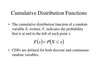
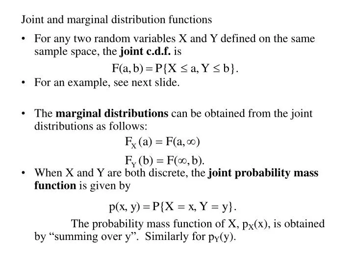
Joint and marginal distribution functions. For any two random variables X and Y defined on the same sample space, the joint c.d.f. is For an example, see next slide. The marginal distributions can be obtained from the joint distributions as follows:

E N D
Joint and marginal distribution functions • For any two random variables X and Y defined on the same sample space, the joint c.d.f. is • For an example, see next slide. • The marginal distributions can be obtained from the joint distributions as follows: • When X and Y are both discrete, the jointprobability mass function is given by The probability mass function of X, pX(x), is obtained by “summing over y”. Similarly for pY(y).
Example for joint probability mass function Y=0 Y=3 Y=4 • Consider the following table: • Using the table, we have X=5 1/7 1/7 1/7 3/7 pX X=8 3/7 0 1/7 4/7 4/7 1/7 2/7 pY
Expected Values for Jointly Distributed Random Variables • Let X and Y be discrete random variables with joint probability mass function p(x, y). Let the sets of values of X and Y be A and B, resp. We define E(X) and E(Y) as • Example. For the random variables X and Y from the previous slide,
Law of the Unconscious Statistician Revisited • Theorem. Let p(x, y) be the joint probability mass function of discrete random variables X and Y. Let A and B be the set of possible values of X and Y, resp. If h is a function of two variables from R2 to R, then h(X, Y) is a discrete random variable with expected value given by provided that the sum is absolutely convergent. • Corollary. For discrete random variables X and Y, • Problem. Verify the corollary for X and Y from two slides previous.
Joint and marginal distribution functions for continuous r.v.’s • Random variables X and Y are jointly continuous if there exists a nonnegative function f(x, y) such that for every well-behaved subset C of lR2. The function f(x, y) is called the joint probability density function of X and Y. • It follows that • Also,
Example of joint density for continuous r.v.’s • Let the joint density of X and Y be • Prove that (1) P{X>1,Y<1} = e–1(1– e–2) (2) P{X<Y} = 1/3 (3) FX(a) = 1 – e–a, a > 0, and 0 otherwise.
Expected Values for Jointly Distributed Continuous R.V.s • Let X and Y be continuous random variables with joint probability density function f(x, y). We define E(X) and E(Y) as • Example. For the random variables X and Y from the previous slide, That is, X and Y are exponential random variables. It follows that
Law of the Unconscious Statistician Again • Theorem. Let f(x, y) be the joint density function of random variables X and Y. If h is a function of two variables from lR2 to lR, then h(X, Y) is a random variable with expected value given by provided the integral is absolutely convergent. • Corollary. For random variables X and Y as in the above theorem, • Example. For X and Y defined two slides previous,
Random Selection of a Point from a Planar Region • Let S be a subset of the plane with area A(S). A point is said to be randomly selected from S if for any subset R of S with area A(R), the probability that R contains the point is A(R)/A(S). • Problem. Two people arrive at a restaurant at random times from 11:30am to 12:00 noon. What is the probability that their arrival times differ by ten minutes or less? Solution. Let X and Y be the minutes past 11:30 am that the two people arrive. Let The desired probability is
Independent random variables • Random variables X and Y are independent if for any two sets of real numbers A and B, That is, events EA ={X A}, EB={Y B} are independent. • In terms of F, X and Y are independent if and only if • When X and Y are discrete, they are independent if and only if • In the jointly continuous case, X and Y are independent if and only if
Example for independent jointly distributed r.v.’s • A man and a woman decide to meet at a certain location. If each person independently arrives at a time uniformly distributed between 12 noon and 1 pm, find the probability that the first to arrive has to wait longer than 10 minutes. Solution. Let X and Y denote, resp., the time that the man and woman arrive. X and Y are independent.
Sums of independent random variables • Suppose that X and Y are independent continuous random variables having probability density functions fX and fY. Then • We obtain the density of the sum by differentiating: The right-hand-side of the latter equation defines the convolution of fX and fY.
Example for sum of two independent random variables • Suppose X and Y are independent random variables, both uniformly distributed on (0,1). The density of X+Y is computed as follows: • Because of the shape of its density function, X+Y is said to have a triangular distribution.
Functions of Independent Random Variables • Theorem. Let X and Y be independent random variables and let g and h be real valued functions of a single real variable. Then (i) g(X) and h(Y) are also independent random variables • Example. If X and Y are independent, then