Discrete Event Control

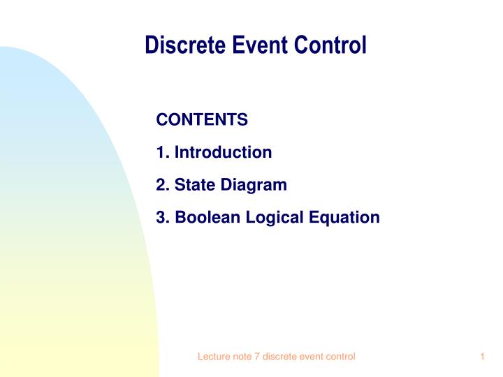
1. Discrete Event Control CONTENTS 1. Introduction 2. State Diagram 3. Boolean Logical Equation Lecture note 7 discrete event control

2. Discrete Event Control 1. Introduction • DEC: both input and output control variable are discrete variables that change values as a result of the occurrence of events • Multiple-input/multiple-output (MIMO) discrete logical controller, see Figure 1, where Ii is discrete value-based input variable, and Yi discrete value-based output. • Ii and Yi only take value 0 (off) or 1 (on). • Input and output devices are usually located at a distance from the controller. Lecture note 7 discrete event control

3. Introduction Figure 1 Y1 I1 Discrete Logic Controller I2 Y2 Ip Ym Lecture note 7 discrete event control

4. Introduction Figure 2 Figure 3 Level Limit LLS V Switch Controller Valve Lecture note 7 discrete event control

5. We need a method to represent system dynamics. Control system: including both plant and controller. However, in discrete event driven system, plant dynamics is ignored. Therefore, the control system for discrete event driven system reduces to the controller only. • State and state diagram is the method. • Next, we discuss state and state diagram. Lecture note 7 discrete event control

6. Is LLS state variable? State Diagram States: indicators that system changes State Variables: assign a name to each independent class of states EX 1: Switch: on and off. (1,0). State change has a cause. State diagram (Fig.4, Fig.5) represents the cause-state change. In particular, node: state; edge: cause. In this example, we define: LLS=0 for the level of liquid is below L LLS=1 for the level of liquid is above L NO Lecture note 7 discrete event control

7. State Diagram State -> System state. System: components: valve, pump. Fluid: is not a part of the system, though the fluid has its state as well. Level of fluid in the tank can be considered as a kind of state, but not in the sense of system state. Since we concern system state, the level of fluid is not considered as a state variable. Level of fluid is input variable in this case; see the next slide. In future, state refers to system state, but we omit word ‘system’ here. Lecture note 7 discrete event control

8. State Diagram Level of fluid: LLS Control system (X: state variable) Remain to see what is X and what is output. Lecture note 7 discrete event control

9. State diagram Figure 4 Figure 5 Lecture note 7 discrete event control

10. State Diagram Level of fluid: LLS Control system (X: state variable) X: state variable: valve Output: X as well So we have: output = X Lecture note 7 discrete event control

11. State Diagram It is noted that the two circles represent different states of one state variable (i.e., valve). The system in EX 1 has only one state variable. EX 2:In EX 1, if we introduce also the pump in the system. In particular, there is a piece of knowledge: when the valve is closed the pump must be off. We can sum up the desired control actions as follows: Lecture note 7 discrete event control

12. State Diagram State variables: X1: pump; X2: valve. X1: X1=0: pump off X1=1: pump on X2: X2=0: valve is closed X2=1: valve is open Lecture note 7 discrete event control

13. State Diagram (for controller) • Open the valve if it is closed and the level of liquid in the tank is less than the desired level L (LLS=0), or keep the valve open if LLS=0. • Close the valve if it is open and the level of liquid in the tank is equal to or greater than the desired level L (LLS=1), or keep the valve closed if LLS=1. • Turn the pump on if it is off and the valve is open and LLS=0, or keep the pump on if it is already on and the valve is open and LLS=0. Lecture note 7 discrete event control

14. State Diagram 4. Turn the pump off if it is on and LLS=1, or keep the pump off if LLS=1. The above expressions of control action can be represented by two state variables, namely X1 (for pump) and X2 (for valve) X1=0, X2=0 (pump off, valve closed) X1=0, X2=1 (pump off, valve open) X1=1, X2=1 (pump on, valve open) Fig.6 shows the state diagram for EX 2. Lecture note 7 discrete event control

15. State Diagram Figure 6 Put all state variables of the system in one circle Lecture note 7 discrete event control

16. State Diagram • Fig. 7 shows another way to represent the state diagram for EX 2. The features of Fig. 7 are: • Each node represents one state variable with its value. • A state variable can be the cause of changes for other state variables. Lecture note 7 discrete event control

17. State Diagram Fig. 7 The meaning that the pump can never be on if the valve is closed has not been represented by the state diagram. This shows some limitation of the state diagram Lecture note 7 discrete event control

18. State Diagram Level of fluid: LLS Control system (X: state variable) X1: state variable: pump X2: state variable: valve Output: X1, X2 So we have: output = X Lecture note 7 discrete event control

19. State Diagram: Summary I O Control system (X: state variable) I: a vector of inputs O: a vector of outputs X: a vector of state variables I and O are in general function of X. In a special case, O=X or I=X. Lecture note 7 discrete event control

20. State Diagram: Summary • State diagram involves logical variables that take 0 or 1 as their values. State diagram has nodes and edges. • Each edge represents one cause or event for the state change in the corresponding nodes. The cause is also a representation of the logical variables. For instance, in Fig. 7, the cause can be written as: X2=1 and LLS =0. • The state diagram has some limitation to express the meaning of the desired control action. A formal way or mathematical way to represent the meaning: If X2=1 AND LLS=0, X1 changes from 0 to 1. This desire leads us to think of Boolean algebra. The idea is to think another way to represent the controller or control system. The next will discuss Boolean algebra. Lecture note 7 discrete event control

21. Boolean Logic Equations Boolean Logic Equations Let A and B be binary variables; that is, A, B=0, or 1. When A =1 (B=1) means that A is true (resp., B is true). A =0 (B=0) means that A is false (resp., B is false). (1) A+B means that either A or B is true A+B=0 when A=0 and B=0 A+B=1 otherwise Lecture note 7 discrete event control

22. Boolean Logic Equation (2) AB means that both A and B are true AB=1 when A=1 and B=1 AB=0 otherwise (3) Not operation, by when A=0 when A=1 Lecture note 7 discrete event control