Download
1 / 29
300 likes | 1.39k Views
Arc-length computation and arc-length parameterization. Arc-length computation. Parametric spatial curve used to define the route of an object Q(t)=(x(t),y(t),z(t)) Arc-length computation necessary for motion control along a curve Control the speed at which the curve is traced

E N D
Arc-length computation • Parametric spatial curve used to define the route of an object Q(t)=(x(t),y(t),z(t)) • Arc-length computation necessary for motion control along a curve • Control the speed at which the curve is traced • Two problems • Parameter t ->arc length s, s=A(t) • Arc length s ->parameter t, t=A-1(s)
Relationship between arc length and parameter • In general, t and s are not linearly related
Analytic approach to computing arc length • Arc length is a geometric integration • In general, this integral doesn’t integrate • Solution: Numeric approaches
Numerical approaches for arc-length computation • Divide the range [t0,t] into intervals • Compute arc length within each interval • Gaussian quadrature • Simpson’s rule • … • Arc length within range [t0,t] computed as the sum of arc length within each interval
Control accuracy of arc length computation • Adaptive method to compute arc length within one interval • Compute arc length within the whole interval, L • Divide the interval into two halves • Compute arc length within each sub interval, L1,L2 • Error is estimated asL – (L1+L2) • Stop, if error is within required accuracy, otherwise, • Repeat above steps for each sub interval
Accelerate arc-length computation • Build a table • Divide the parameter range into intervals • Compute arc length within each interval • Build a table of correspondence between parameter and arc length • Map parameter to arc length • Map parameter to an interval • Find arc-length value before this interval from the table • Compute the arc length within part of the interval
Traditional approach of arc-length parameterization for parametric curves • Compute arc length s as a function of parameter t s=A(t) • Compute the inverse of the arc-length function t=A-1(s) • Replace parameter t in Q(t)=(x(t),y(t),z(t)) with A-1(s)
Numerical arc-length parameterization (cont.) • Bisection method to compute t=A-1(s) • Table search to locate an interval [ti, ti+1] , A(ti ) ≤s <A(ti+1 ) • Use [ti, ti+1] as the start interval • Each iteration an arclength integration evaluated • Advantage: solution guaranteed • Problem: slow and lots of computations
Numerical arc-length parameterization (cont.) • Newton-Raphson method to compute t=A-1(s) • Seen as root finding problem of the equation, f(t)=s-A(t)=0 • Table search to locate an interval • Linear interpolation within the interval to compute • Compute sequence of ,
Numerical arc-length parameterization (cont.) • Advantage of Newton-Raphson method • May faster than bisection method, although no guarantee • Problems: • Each iteration an arc-length integration evaluated • Ti may lie outside the definition of the space curve • no guarantee of convergence
Use explicit function to approximate arc-length parameterization • Functions relate arc-length s and parameter t • s strictly monotonically increasing with t • A curve describes how s varies with t, s=A(t) • t strictly monotonically increasing with s • A curve describes how t varies with s, t=A-1(s) • Bezier curves are an option
Use explicit function to approximate arc-length parameterization (Cont.) • The four control points of a Bezier curve • , • By linear precision property, • A(1/3) & A(2/3) computed from original curve • Solve & from 2 equations
Use explicit function to approximate arcle-ngth parameterization (Cont.) • Two-span Bezier curve • Two-span Bezier curve used when A(t) has more than one inflexion points • If A(t) has 2 inflexion point t1 and t2, the break point of the two spans is in (t1 +t2)/2 • If A(t) has 3 inflexion point t1, ,t2 and t3 , the break point of the two spans is t2
Use explicit function to approximate arc-length parameterization (Cont.) • Advantages • Fast function evaluations • Constant time to compute t from s • Constant time to compute s from t • Disadvantages • Error out of control • Numerical root finding to locate inflexion points • No guarantee of monotonicity
Arc-length parameterization in Hank • Roads modeled as ribbons with centerline modeled as cubic spline Q(t) • Curvilinear coordinates • ,distance on centerline from start point • ,offset from centerline • ,loft from road surface • Mapping between and (x,y,z) in real time
Approximately arc-length parameterized cubic spline curve • Compute curve length • Find m+1 equally spaced points on input curve • Interpolate (x,y,z) to arc length s to get a new cubic spline curve
Compute arc length and build a mapping table • Compute arc length of a cubic spline piece with Simpson’s rule • Adaptive methods can be used to control the accuracy of arc length computation • Lengths of all spline pieces are summed • Build a table for mappings between parameter and arc length on knot points
Find m+1equally spaced points • Problem • Mappings from equally spaced arc-length values 0, 1L/m, 2L/m, …, mL/m to parameter values • Solution: • Table search to map an arc-length value to a parameter interval • Bisection method to map the arc-length value to a parameter value within the parameter interval
Compute an approximate arc-length parameterized spline curve • m+1 points as knot points • Arc length as parameter • Using cubic spline interpolation • End point derivative conditions, or, • Not-a-knot conditions • Endpoint derivative conditions • Direction of tangent vector on end points consistent with the input curve • Magnitude of tangent vector on end points is 1.0
Errors • Match error • Misfit of the derived curve from an input curve • Arc-length parameterization error • deviation of the derived curve from arc-length parameterization
Errorsanalysis • Match error • Traverse the derived curve and input curve • Match error is the difference between two curves at corresponding points, |Q(t)-P(s)| • Arc-length parameterization error • For an arc-length parameterized curve, • Arc-length parameterization error measured by
Experimental results (1) Experimental curve (2) Curvature of the curve
Experimental results (cont.) (1) m=5 (2) m=10 Experimental curve(blue) and the derived curve (red) with their knot points
Experimental results (cont.) (1) m=5 (2) m=10 Match error of the derived curve
Experimental results (cont.) (1) m=5 (2) m=10 Arc-length parameterization error of the derived curve
Error factors in experimental results • Both errors increase with curvature • Both errors decrease with m • Maximal match error decreases 10 times when m doubled • Maximal arc-length parameterization error decreases 5 times when m doubled
Strengths of this technique • Run-time efficiency is high • No mapping between parameter and arc-length needed • No table search needed for mapping from curvilinear coordinates to Cartesian coordinates • Mapping form Cartesian coordinates to curvilinear coordinates is efficient (introduced in another paper) • Time-consuming computations can be put either in initialization period or off-line
Strengths of this technique (cont.) • Higher accuracy can be achieved • By computing length of the input curve more accurately • By locating equal-spaced points more accurately • By increasing m • Burden of higher accuracy is only more memory • Doubling m requires doubling the memory for spline curve coefficients