Download
1 / 60
610 likes | 1.15k Views
Modelling and Measuring Price Discovery in Commodity Markets. Isabel Figuerola-Ferretti Jesús Gonzalo Universidad Carlos III de Madrid Business Department and Economics Department December 2007. Trading Places Movie. Two Whys.

E N D
Modelling and Measuring Price Discovery in Commodity Markets Isabel Figuerola-Ferretti Jesús Gonzalo Universidad Carlos III de Madrid Business Department and Economics Department December 2007
Two Whys • There are two standard ways of measuring the contribution of financial markets to the price discovery process: (i) Hasbrouck (1995) Information Shares (ii) Gonzalo and Granger (1995) P-T decomposition, suggested by Harris et al. (1997) We want to find a THEORETICAL JUSTIFICATION for the USE of GGP-Tdecomposition for price discovery. • Can the cointegrating vector be different from (1, -1)? Empirically Yes; but theoretically? YES, TOO.
Other minor Whys • Why Price Discovery? Markets have two important functions: Liquidity and Price Discovery, and these functions are important for asset pricing. • Why Commodities? Commodities, in sharp contrast to more traditional financial assets, are more tied to current economic conditions. • Why Metals? The chief market place is the London Metal Exchange (LME).
Road Map • Introduction • Equilibrium Model of Commodity St and Ft Prices with Finite Elasticity of Arbitrage Services + Convenience Yields (built on Garbade and Silver (1983)) • Econometric Implementation : Theoretical model and the GG P-T decomposition • Data (London Metal Exchange : Al, Cu, Ni, Pb, Zn) • Results (Backwardation; and dominant markets in the price discovery process) • Conclusions
Introduction Future markets contribute in three important ways to the organization of economic activity: • they facilitate price discovery • they provide an arena for speculation • they offer means of transferring risk or hedging.
Introduction Price discovery is the process by which security or commodity markets attempt to identify permanent changes in equilibrium transaction prices. • The unobservable permanent price reflects the fundamental value of the stock or commodity. • It is distinct from the observable price, which can be decomposed into its fundamental value and its transitory effects (due to the bid-ask bounce, temporary order imbalances, inventory adjustments, etc)
Introduction For producers as well as consumers it is important to determine where the price information and price discovery are being produced. More on Price Discovery: • The process by which future and cash markets attempt to identify permanent changes in equilibrium transaction prices. • If we assume that the spot and future prices measure a common efficient price with some error, price discovery quantifies the contribution of spot and future prices to the revelation of the common efficient price.
IntroductionSpecific Contributions: • We extend the equilibrium model of the term structure of commodity prices developed by Garbade and Silver (1983) (GS) by incorporating endogenously convenience yields. This allows us to capture the existence of Backwardationand Contango. This is reflected on a cointegrating vector (1, -b2), different from the standard and always present b2 =1. When b2 >1 (<1) the market is under backwardation (contango). • Independent of b2 , we prove that the equilibrium model can be written as an error correction model, where the permanent component of the GG P-T decomposition coincides with the price discovery process of GS. This justifies theoretically the use of this type of decomposition. • All the results in the paper are testable, as it can be seen in the application to non-ferrous metal markets: (i) All the markets are in Backwardation but Copper (ii) For those metals with highly liquid future markets, future prices are the dominant factor in the price discovery process.
Literature Review 1:Literature on price discovery • Garbade, K. D. & Silver W. L. (1983). Price movements and price discovery in futures and cash markets. Review of Economics and Statistics. 65, 289-297. • Hasbrouck, J. (1995). One security, many markets: Determining the contributions to price discovery. Journal of Finance 50, 1175-1199. • Harris F. H., McInish T. H., Wood R. A. (1997).”Common Long-Memory Components of Intraday Stock Prices: A Measure of Price Discovery.” Wake Forest University Working Paper.
Literature Review 2:Price discovery metrics • Hasbrouck, J. (1995). One security, many markets: Determining the contributions to price discovery. Journal of Finance 50, 1175-1199. • Gonzalo, J. Granger C. W. J (1995). Estimation of common long-memory components in cointegrated systems. Journal of Business and Economic Statistics 13, 27-36.
Literature Review 3Comparing the two metrics of price discovery:Special Issue Journal of Financial Markets 2002 • Baillie R., Goffrey G., Tse Y., Zabobina T. (2002). Price discovery and common factor models. • Harris F. H., McInish T. H., Wood R. A. (2002). Security price adjustment across exchanges: an investigation of common factor components for Dow stocks. • Hasbrouck, J. (2002). Stalking the “efficient price” in market microstructure specifications: an overview. • Leathan Bruce N. (2002). Some desiredata for the measurement of price discovery across markets. • De Jong, Frank (2002). Measures and contributions to price discovery: a comparison.
Theoretical Model: Extension of Garbade and Silber (1983) Equilibrium with infinitely elastic supply of arbitrage • St = Log of the spot market price at time “t” • Ft = Log of the contemporaneous price on a futures contract for a commodity for settlement after a time interval T1= T-t (e.g. 15 months) • rt interest rate applicable to the interval from t to T.
Equilibrium with infinitely elastic supply of arbitrage Standard Assumptions: 1) No taxes or transaction cost 2) No limitations on borrowing 3) No costs other than financing + storage a (short or long) future position 4) No limitations on short sale of the commodity in the spot market 5) Interest rate rt + storage cost ct = + I(0), with the mean of (rt + ct) 6) St is I(1).
Equilibrium with infinitely elastic supply of arbitrage • Let T1=1 • Non-arbitrage equilibrium conditions imply • Given the above assumptions, equation (1) implies that St and Ft are cointegrated with the always present cointegrating vector (1, -1).
A bit of more realism: Convenience Yields In consumption commodities is very likely that with where is the convenience yield. Convenience yield is the flow of services that accrues to an owner of the physical commodity but not to an owner of a contract for future delivery of the commodity (Brennan Schwartz (1985) ). The existence of convenience yields can produce two situations very common in commodity markets: BACKWARDATION and CONTANGO.
Convenience Yields One more Assumption: 7) The convenience yield is modeled as with .
Backwardation refers to futures prices that decline with time to maturity • Contango refers to futures prices that rise with time to maturity
Equilibrium with convenience yields • Substituting (3) into (2) + (a.5) with and . It is important to notice the different values that 2 can take • 1) 2>1 then 1>2 . In this case we are under the process of long-runbackwardation (“St>Ft” in the long-run) • 2) 2=1 then 1=2. In this case we do not observe long-runbackwardation or contango • 3) 2<1 then 1<2 . In this case we are under the process of long-run contango (“St<Ft” in the long-run)
Equilibrium with convenience yields Some remarks: • The parameters 1 and 2 are not identified in the equilibrium equation (4) unless is known, or for instance we impose 1 + 2 =1. In the fomer case: 1 = 1+rc/ β3 and 2 = 1- β2 (1- 1 ). • Convenience yields are stationary when β2 =1. When β21 it contains a small random walk component. The size depends on the difference (2 -1).
Equilibrium with finitely elastic supply of arbitrage services In realistic cases we expect the arbitrage transactions of buying in the cash market and selling the futures contracts or vice versa not to be riskless: unknown transaction costs, unknown convenience yields, constraints on warehouse space, basis risk, etc. These are the cases of finite elasticity of arbitrage services. To describe the interaction between cash and future prices we must first specify the behaviour of agents in the marketplace. • There are Ns participants in spot market. • There are Nf participants in futures market. • Ei,t is the endowment of the ith participant immediately prior to period t. • Rit is the reservation price at which that participant is willing to hold the endowment Ei,t. • Elasticity of demand, the same for all participants.
Equilibrium with finitely elastic supply of arbitrage services • Demand schedule of ith participant in spot market where A is the elasticity of demand • Aggregate cash market demand schedule of arbitrageurs in period t where H is the elasticity of cash market demand by arbitrageurs. It is finite when the arbitrage transactions of buying in the cash market and selling the futures contract or vice versa are not riskless.
The cash market will clear at the value of St that solves • The future market will clear at the value of Ft such that
Equilibrium with finitely elastic supply of arbitrage services • Solving the clearing market conditions as a function of the mean reservation pricesand
Dynamic price relationships • To derive dynamic price relationships, we need a description of the evolution of reservation prices.
Dynamic price relationships: VAR model where and Garbade and Silver (with b2=1, b3=0) stop their analysis at this point stating that Measures the importance of future markets relative to cash markets
The GG permanent component is… This is our price discovery metric, which coincides with the one proposed by GS. Our metric does not depend on the existence of backwardation or contango.
Two extreme cases: • H = 0 No VECM, no cointegration. Spot and Future prices will follow independent randon walks. This eliminates both the risk transfer and the price discovery functions of future markets • H = ∞ In VAR (12) the matrix M has reduced rank (1, -2)M =0 , and the errors are perfectly correlated. Therefore the long run equilibrium relationship (4), St= 2 Ft + 3, becomes an exact relationship. Future contracts are in this situation perfect substitutes for spot market positions and prices will be “discovered” in both markets simultaneously.
Two Metrics for Price Discovery:IS of Hasbrouck (1995) and PT of Gonzalo and Granger (1995) • See Special Issue of the Journal of Financial Markets, 2002, 5 • Both approaches start from the estimation of the VECM • Hasbrouck transforms the VECM into a VMA with Y denoting the common row vector of Y(1) and l a column unit vector.
Two Metrics for Price Discovery:IS of Hasbrouck (1995) and PT of Gonzalo and Granger (1995) • The information share (IS) measure is a calculation that attributes the source of variation in the random walk component to the innovations in the various markets. To calculate it we need to have uncorrelated innovations: ut=Qet, with Var(ut)=W=QQ’ and Q a lower triangular matrix (Choleski decomposition of W ) • The market-share of the innovation variance attributable to ej is where [YQ]j is the j-th element of the row matrix YQ.
Some Comments on the IS metric • Non-uniqueness. There are many square roots of W and not even the Cholesky square root is unique. Solution: To calculate all the Choleskys, and form upper and lower bounds of the IS. Problem: Theses bounds can be very distant. (2) It is not clear how to proceed when the cointegrating vector is different from (1, -1). • It presents some difficulties for testing (4) Economic Theory behind it???
PT of GG P-T decomposition where It exists if det(b’a) different from zero.
Some Comments on GG PT Advantages: • The linear combination defining Wt is unique • Easy estimation (by LS) • Easy testing (chi-squared distribution) • Economic Theory behind it (well not always ha ha ha ha). Problems: • It needs to invert a matrix so it may not exist (probability zero) • Wt may not be a random walk; but it can be.
Empirical Price Discovery in non Ferrous Metal Markets.Data • Daily spot and future (15 months) for Al, Cu, Ni, Pb, Zn, quoted in the LME • Sample January 1989- October 2006 • Source Ecowin. The LME data has the advantage that there are simultaneous spot and forward ask prices, for fixed maturities, every business day.
Empirical Price Discovery in non ferrous metal markets Six Simple Steps : 1) Perform unit root test on price levels 2) Determine the rank of cointegration 3) Estimation of the VECM 4) Hypothesis testing on beta 5) Estimation of α and hypothesis testing on it (e.g. α ´=(0, 1)) 6) Set up the PT decomposition.
Conclusions and Extensions • We introduce a way of modelling endogenously convenience yields, such that Backwardation and Contango are captured in the cointegrating vector. Cointegrating vector that is different from the standard and always present (1, -1) • As a by-product we can calculate convenience yields • An Economic Theoret¡cal justification for the GG PT decomposition • For those metals with most liquid future markets the future price is the major contributor to the revelation of the efficient price (price discovery). This means that for those commodities producers and consumers should rely on the LME future price to make their production and consumption decisions • On going extensions : (1) To other commodities (2) Backwardation and contango jointly in the model. This will imply a non-linear ECM.