Download
1 / 10
120 likes | 210 Views
Gain an insight on our Quantitative Analysis by statistic experts of EssayCorp across the world. We guarantee plagiarism free work. For any academic help contact us at contact@essaycorp.com. We also provide urgent projects at ease.

E N D
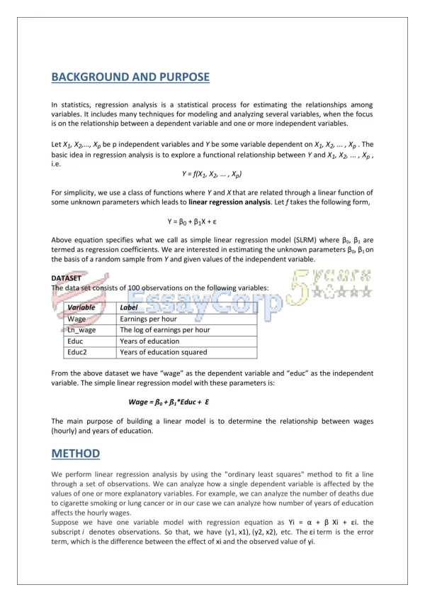
BACKGROUND AND PURPOSE In statistics, regression analysis is a statistical process for estimating the relationships among variables. It includes many techniques for modeling and analyzing several variables, when the focus is on the relationship between a dependent variable and one or more independent variables. Let X1, X2,..., Xp be p independent variables and Y be some variable dependent on X1, X2, ... , Xp . The basic idea in regression analysis is to explore a functional relationship between Y and X1, X2, ... , Xp , i.e. Y = f(X1, X2, ... , Xp) For simplicity, we use a class of functions where Y and Xthat are related through a linear function of some unknown parameters which leads to linear regression analysis. Let f takes the following form, Y = β0+ β1X + ε Above equation specifies what we call as simple linear regression model (SLRM) where β0, β1 are termed as regression coefficients. We are interested in estimating the unknown parameters β0, β1 on the basis of a random sample from Y and given values of the independent variable. DATASET The data set consists of 100 observations on the following variables: Variable Label Wage Earnings per hour Ln_wage The log of earnings per hour Educ Years of education Educ2 Years of education squared From the above dataset we have “wage” as the dependent variable and “educ” as the independent variable. The simple linear regression model with these parameters is: Wage = ß0 + ß1*Educ + Ɛ The main purpose of building a linear model is to determine the relationship between wages (hourly) and years of education. METHOD We perform linear regression analysis by using the "ordinary least squares" method to fit a line through a set of observations. We can analyze how a single dependent variable is affected by the values of one or more explanatory variables. For example, we can analyze the number of deaths due to cigarette smoking or lung cancer or in our case we can analyze how number of years of education affects the hourly wages. Suppose we have one variable model with regression equation as Yi = α + βXi + εi.the subscript i denotes observations. So that, we have (y1, x1), (y2, x2), etc. The εi term is the error term, which is the difference between the effect of xi and the observed value of yi.
The OLS works on the principle of minimizing the sum of squares more specifically the squared error terms. We need to minimize the 2 variables with respect to α and ß. Thus we have: After solving we get, These are called the OLS estimators of α and ß respectively. So the fitted value of y can be obtained by and the residuals can be obtained as SIMPLE LINEAR REGRESSION ANALYSIS To examine the relationship between ‘education’ (the independent variable) and ‘wage’ (the dependent variable), we examine: a)Summary statistics and histograms: Descriptive Statistics Range Min Max Mean Median Mode . Std Dev Var Skewness Kurtosis 22.31 14.02 1.49 2.61 72.06 4.33 76.39 19.39 7.50 196.60 WAGE EDUC 13.76 2.73 0.44 1.32 15 6 21 13 12 7.44 From the summary statistics we can infer that the mean wage and mean education years are 22.31 13.76, means that their respective data is clustered around these averages. Also the standard deviation of wage 14.02 describes high dispersion in data from the mean value and the standard deviation of education 2.73 describes lesser dispersion in data from the mean value. This means the data for education is much closely packed as compared to the wages. Skewness of wage approx 1.5 which tells that the data might be positively skewed whereas skewness for education is approx 0 which means data might be symmetrical. Also the kurtosis of both wage and education tell that curve will be platykurtic in nature. The histograms for wages and education are given below:
b)Estimate the linear regression model wage = ß1 + ß2* educ + ε and interpret the slope: Below is the model summary for the simple regression model, Regression Statistics Multiple R R Square Adjusted R Square Standard Error Observations The Multiple R represents the simple correlation between the two variables. Here multiple R is 0.413 which not very high i.e., low degree of correlation. R Square represents the total variation in the dependent variable wage that can be explained by the independent variable education. In this case only 17.1%, which is quite low. 0.413 0.171 0.162 12.834 100 Next is the ANOVA Table, ANOVA df SS MS F Sig F 0.000 Regression Residual Total 1 3320.694 16142.777 19463.470 3320.694 164.722 20.159 98 99 This table indicates that the regression model predicts the dependent variable significantly well. We know this from the "Regression" row and "Sig." column. This indicates the statistical significance of the regression model that was run. Here, p = 0.000, which is less than 0.05 (5% level of significance), and indicates that, overall, the regression model statistically significantly predicts the outcome variable (i.e., it is a good fit for the data). We may note that even though the R2 value was very low still the model is a good fit. Now, we have the coefficients table, Standard Error P- t Stat -1.042 4.490 Coefficients -6.915 value 0.300 0.000 Intercept Educ 6.634 0.473 2.124 The Coefficients table provides us with the necessary information to predict wages from education, as well as determine whether education contributes statistically significantly to the model (by
looking at the "Sig." column). In this case, education contributes significantly to the model. Furthermore, we can use the values to present the regression equation as: Wages = -6.915 + 2.124 * Educ Let's take a look at our regression equation. In this scenario we have 2.124 as the slope and -6.195 as the intercept. We know that the slope is the consistent change, or the relationship between two variables, in a linear model. Since the slope coefficient is positive means wages and education hold a positive relation. Also with an increase of 1 year in the education the wages will increase by approximately 2.124 units. A marginal effect of an independent variable x is the partial derivative, with respect to x, of the prediction function f ( dependent function y). Marginal Effect of x on y = The marginal effect of education on wage is the derivative ß2 for the given simple linear regression model, and it is independent of the years of education or addition in the years of education. So, the marginal effect of education on wage for any number of years of education will be 2.124 c)Calculate the residuals and plot them against EDUC. Are any patterns evident and, if so, what does this mean? Below is the table of residuals of all 100 observations, Obs. Residuals Obs. Residuals Obs. 1 -4.410 26 -0.570 2 -6.865 27 -19.865 3 6.202 28 -8.940 4 1.530 29 11.812 5 4.556 30 -4.070 6 7.137 31 3.060 7 -1.464 32 -14.065 8 18.930 33 -2.895 9 -4.320 34 11.937 10 19.095 35 -2.570 11 -3.015 36 7.147 12 8.430 37 -9.394 13 6.430 38 17.060 14 -10.235 39 -6.194 15 -7.835 40 -1.570 16 -12.634 41 0.456 17 -4.820 42 17.805 18 -7.570 43 -5.363 19 -10.785 44 -5.470 20 -12.088 45 3.356 21 -24.933 46 8.830 22 1.060 47 -6.570 23 21.485 48 -9.144 24 1.186 49 -8.570 25 -0.694 50 16.185 Residuals Obs. Residuals 53.560 76 -22.313 77 11.385 78 -4.765 79 2.935 80 26.985 81 -9.570 82 -9.940 83 8.136 84 -1.818 85 -9.944 86 2.910 87 9.066 88 6.430 89 15.196 90 -8.947 91 -12.718 92 -12.170 93 7.530 94 -9.070 95 -10.318 96 -5.120 97 -7.714 98 -13.194 99 10.422 100 53.572 -2.435 4.665 4.430 -5.745 -2.320 20.065 8.985 -16.313 -9.070 -0.710 -3.268 12.932 -7.823 -3.040 2.386 13.606 -3.268 -1.070 0.180 -10.694 -11.430 -14.174 -8.854 -14.318 51 52 53 54 55 56 57 58 59 60 61 62 63 64 65 66 67 68 69 70 71 72 73 74 75
Below is the plot between the residuals and education. The data points appear to be a time series data but it is not. It is just a volatile data with eratic behaviour of residuals. Also, it is difficult to comment on the specific shape of the residuals we cannot infer about the homoscedasticity or hetroscedasticity. d)Estimate the quadratic regression WAGE = α1+ α2EDUC2+ ε and interpret the results. Estimate the marginal effect of another year of education on wage for a person with 12 years of education, and for a person with 14 years of education. Compare these values to the estimated marginal effect of education from the linear regression in part (b). Below is the model summary for the quadratic regression model, Regression Statistics Multiple R R Square Adjusted R Square Standard Error Observations The Multiple R represents the simple correlation between the two variables. Here multiple R is 0.413 which not very high i.e., low degree of correlation. R Square represents the total variation in the dependent variable wage that can be explained by the independent variable education. In this case only 17.1%, which is quite low. 0.413 0.171 0.162 12.834 100 Next is the ANOVA Table, ANOVA df 1 98 99 SS MS F Sig F 0.000 Regression Residual Total 3305.745 16157.725 19463.470 3305.745 164.875 20.050
This table indicates that the regression model predicts the dependent variable significantly well. We know this from the "Regression" row and "Sig." column. This indicates the statistical significance of the regression model that was run. Here, p = 0.000, which is less than 0.05 (5% level of significance), and indicates that, overall, the regression model statistically significantly predicts the outcome variable (i.e., it is a good fit for the data). We may note that even though the R2 value was very low still the model is a good fit. Now, we have the coefficients table, Std Error 3.449 0.016 t Stat 2.313 4.478 Coefficients 7.976 0.073 P-value 0.023 0.000 Intercept educ2 The Coefficients table provides us with the necessary information to predict wages from education, as well as determine whether education contributes statistically significantly to the model (by looking at the "Sig." column). In this case, education contributes significantly to the model. Furthermore, we can use the values to present the regression equation as: Wages = 7.976 + 0.073 * Educ2 Let's take a look at our regression equation. In this scenario we have 0.073 as the slope and 7.976 as the intercept. We know that the slope is the consistent change, or the relationship between two variables, in a linear model. Since the slope coefficient is positive means wages and education hold a positive relation. Also with an increase of 1 year in the education the wages will increase by approximately 0.073 units. A marginal effect of an independent variable x is the partial derivative, with respect to x, of the prediction function f ( dependent function y). Marginal Effect of x on y = The marginal effect of education on wage is the derivative 2*α2*education for the quadratic regression model, and it varies with the number of years of education. For 12 years of education, the marginal calculation should therefore be 2*0.073*12 = 1.752 For 14 years of education, the marginal calculation should therefore be 2*0.073*14 = 2.044 The marginal effect of another year of education on wage for a person with 12 years of education, will be 0.073*13*13-0.073*12*12 = 1.825 The marginal effect of another year of education on wage for a person with 14 years of education, will be 0.073*15*15-0.073*14*14 = 2.117 Although we must note that the comparison of the wage at 12, 13 years and 14, 15 years of education is only an approximation to the marginal effect of 12 and 14 years. A more accurate approximation can be obtained by comparing (12.1 and 12) and (14.1 and 14). When these values are compared to the estimated marginal value for simple linear regression model we can observe that the estimated marginal value for SLRM is a constant i.e., independent of the effect of years of education on wage whereas in quadratic regression model with a unit increase in education the wages increases by 2*0.073 units.
e)Construct a histogram of ln(WAGE). Compare the shape of this histogram to that for WAGE from part (a). Which appears to be more symmetric and bell- shaped? The histograms for ln(wage) and wage are given below, The histogram of wage depicts that the data might be positively skewed. But we can observe in the histogram of ln(wage) that it is more symmetric and bell shaped.
f)Estimate the log-linear regression ln(WAGE) = γ1 + γ2EDUC + ε and interpret the slope. Estimate the marginal effect of another year of education on wage for a person with 12 years of education, and for a person with 14 years of education. Compare these values to the estimated marginal effects of education from the linear regression in part (b) and quadratic in part (d) Below is the model summary for the simple regression model, Regression Statistics Multiple R R Square Adjusted R Square Standard Error Observations The Multiple R represents the simple correlation between the two variables. Here multiple R is 0.424 which not very high but higher than the R obtained in SLRM and quad regression model. R Square represents the total variation in the dependent vbl wage that can be explained by the independent variable education. In this case only 18%, which is also higher than the R2 obtained in the other 2 models. 0.424 0.180 0.171 0.545 100 Next is the ANOVA Table, ANOVA df SS 6.375 29.099 35.474 MS 6.375 0.297 F Sig F 0.000 Regression Residual Total 1 21.468 98 99 This table indicates that the regression model predicts the dependent variable significantly well. We know this from the "Regression" row and "Sig." column. This indicates the statistical significance of the regression model that was run. Here, p = 0.000, which is less than 0.05 (5% level of significance), and indicates that, overall, the regression model statistically significantly predicts the outcome variable (i.e., it is a good fit for the data). Now, we have the coefficients table, Std Error t Stat 5.852 4.633 Coefficients P-value 0.000 0.000 Intercept Educ 1.648 0.093 0.282 0.020 The Coefficients table provides us with the necessary information to predict wages from education, as well as determine whether education contributes statistically significantly to the model (by looking at the "Sig." column). In this case, education contributes significantly to the model. Furthermore, we can use the values to present the regression equation as: Ln(Wages) = 1.648 + 0.093 * Educ Let's take a look at our regression equation. In this scenario we have 0.093 as the slope and 1.648 as the intercept. We know that the slope is the consistent change, or the relationship between two variables, in a linear model. Since the slope coefficient is positive means wages and education hold a
positive relation. Also with an increase of 1 year in the education the wages will increase by approximately 0.093 units. The marginal effect of the given log linear regression model will be given as: Ln (wage) = γ0+ γ1 * education Wage = exp ( γ0+ γ1 * education ) Marginal Effect of x on y = 2 * For 12 years of education, the marginal effect is 0.093*exp(1.648+0.093*12)= 1.475 For 14 years of education, the marginal effect is 0.093*exp(1.648+0.093*14)= 1.776 The marginal effect of another year of education on wage for a person with 12 and 14 years of education is independent of the number of years of education, given as = exp(γ1)= 1.097 On comparing and summarizing the results obtained in the 3 regressions performed, we find that the marginal effect of education on wage for simple linear regression model is independent of the years of education and is equal to the coefficient ß2 = 2.124. For the quadratic regression model the marginal effect of another year of education on wage for a person with 12 years of education is 1.825 and for 14 years of education is 2.117. And for log linear model, the marginal effect for 12 years of education is 1.475 and 14 years of education is 1.776. Also the marginal effect of another year of education on wage for a person is independent of the years of education and is 1.097. RECOMMENDATION After analyzing the three models in the above study, it can be recommended that log linear regression model should be used instead of simple linear or quadratic regression model as it provides better fit to the data as the ln(wage) is symmetric and bell shaped, higher variability is explained and it fits better to the data as compared to the other two models.
REFRENCES 1.Gupta and Kapoor, Fundamentals Of Mathematical Statistics, Sultan Chand and Sons, 1970. 2.Gupta and Kapoor, Fundamentals Of Applied Statistics, Sultan Chand and Sons, 1970. 3.Chatterjee, S. and Price, B. Regression Analysis by Example. Wiley, New York, 1977. 4.Darius Singpurwalla, A Handbook Of Statistics, An overview of statistical methods, 2013. 5.Mosteller, F., & Tukey, J. W., Data analysis and regression: A second course in statistics. Reading, MA: Addison-Wesley, 1977. 6.Anon, (2016). [online] http://www.law.uchicago.edu/files/files/20.Sykes_.Regression.pdf [Accessed 12 Jan. 2016]. 7.Anon, (2016). [online] https://www.youtube.com/watch?v=_Rudt0ivG74. [Accessed 12 Jan. 2016]. 8.Anon, (2016). [online] http://www.123helpme.com/search.asp?text=regression+analysis [Accessed 12 Jan. 2016]. Available at: - Available at: - Available at: -