Download
1 / 57
630 likes | 825 Views
FPGA Accelerated 3-D Tomography. Richard Dorrance Progress Update: 09/07/12. Outline. Introduction to Tomography Reconstruction Methods Analytical Backprojection Filtered Backprojection Algebraic Algebraic Reconstruction Technique (ART)

E N D
FPGA Accelerated3-D Tomography Richard Dorrance Progress Update: 09/07/12
Outline • Introduction to Tomography • Reconstruction Methods • Analytical • Backprojection • Filtered Backprojection • Algebraic • Algebraic Reconstruction Technique (ART) • Simultaneous Iterative Reconstruction Technique (SIRT) • Simultaneous Algebraic Reconstruction Technique (SART) • Modeling Performance of Reconstruction Methods • Future Work
Tomography • Cross-sectional imaging technique using transmissionor reflection data from multiple angles • Basis for CAT scan, MRI,PET, SPECT, ET, etc. • Computed Tomography (CT):A form of tomographic reconstruction on computers
Cross-Sections by X-Ray Projections • Project X-ray through biological tissue;measure total absorption of ray by tissue • Projection Pθ(t) is the Radontransform of object functionf(x,y): • Total set of projections calledsinogram
Shepp-Logan Phantom • Standard test image for tomographic reconstructions
CT Reconstruction • Restore image from projection data • Inverse Radon transform • Most common algorithm is filtered backprojection • “Smear” each projection over image plane • Accuracy of reconstruction depends on the number of detectors and projection angles Original 4 Angles 16 Angles 64 Angles 256 Angles
Analytical Reconstruction Methods • (Filtered) Backprojection Pseudo Code: • Input: sinogram sino(θ, N) • Output: image img(x,y) for each θ filter sino(θ,:) ; only for FBP for each x for each y n = x*cos(θ)+ y*sin(θ) img(x,y)= sino(θ,n)+ img(x,y)
Backprojection vs. Original • Final Step: normalize image power • Divide each pixel by θ·N
Note On Filtering No Filtering With Filtering
Problem Formulation • We want to formulate it as a Linear Inverse Problem: • Where x is a column vector of length N2 representing the pixels of the original image, A is an M by N2 matrix representing the data acquisition process, and b is a column vector of length M representing the measured projection data. • We want to find a solution such that:
Notes on the Discretized Image x • The discretized image is denoted by:and by:where x is obtained by stacking the columns of X.
Notes on the projection data b • There are a total of d detectors and θ projection angles, so that a total of M = d · θare used. • Then the measured projection data is denoted by:and by:where b is obtained by stacking the columns of B.
Notes on the Acquisition Matrix A • The acquisition of projection data b from x is modeled by:where: • ai,j is the contribution of pixel j to projection i. • Also, let:be a column matrix that represents the ith ray which computes the value of the ith projection.
Iterative Reconstruction Algorithm • Let x(k) denote the kth estimation of the reconstruction. • Then:where the relaxation factor λ is a scalar.
Proof of Convergence [1] • Let • Then
Proof of Convergence [2] • If ATA is positive definite and λ is chosen so that the spectral radius of Δ is less than 1, then:and
Proof of Convergence [3] • Therefore:
# of Projections needed for ART • Reconstruction on a square grid (N×N) with N detectors • Assuming a circular reconstruction region, we can ignore pixels outside this region
# of Projections needed for FBP [1] • Reconstructing region with diameter L • Sampling interval is at least:with a maximum frequency of: • Due to polar sampling,the density of samplesdecreases as we gooutward on the polar grid
# of Projections needed for FBP [2] • To ensure a sampling rate of at least Δω everywhere:therefore:
Matrix Formulation with Normalization • Introduce diagonal matrices V and W: • V: diagonal matrix of theinverse of the row sums • W: diagonal matrix of theinverse of the column sums
Reconstruction Methods • Algebraic Reconstruction Technique • Update image after each ray is processed • Simultaneous Iterative Reconstruction Technique • Update image after all rays are processed • Simultaneous Algebraic Reconstruction Technique • Update image after all rays in a single projection angle are processed
ART • Image update method: • After each ray is processed • Pseudocode: for k = 1:K for i = 1:M end end
SIRT • Image update method: • After all rays are processed • Pseudocode: for k = 1:K end
SART • Image update method: • After all rays in a single projection angle are processed • Pseudocode: for k = 1:K forθ = 1:Θ end end
Modeling Performance (CPU, GPU, FPGA) • Write C pseudo code for Matrix-Vector multiplication and Vector-Vector addition • Convert C pseudo code to application specific pseudo code (CPU = x86, GPU = OpenCL/CUDA) • Model latency and throughput of pseudo code given: • CPU architecture: • Cache structure, freq., total # of threads, etc… • Image reconstruction problem: • N, d, θ, A matrix sparsity (α), # of iterations, etc…