Download

1 / 42
530 likes | 863 Views
Divide and Conquer . Chapter 2. Objectives. Describe the divide-and-conquer approach to solving problems Apply the divide-and-conquer approach to solve a problem Determine when the divide-and-conquer approach is an appropriate solution approach

E N D
Divide and Conquer Chapter 2
Objectives • Describe the divide-and-conquer approach to solving problems • Apply the divide-and-conquer approach to solve a problem • Determine when the divide-and-conquer approach is an appropriate solution approach • Determine complexity analysis of divide and conquer algorithms • Contrast worst-case and average-case complexity analysis
Battle of Austerlitz – December 2, 1805 • Napoleon split the Austro-Russian Army and was able to conquer 2 weaker armies • Divide an instance of a problem into 2 or more smaller instances • Top-down approach
Divide and Conquer • In this approach, a problem is divided into sub-problems and the same algorithm is applied ( usually recursively) to every sub-problem • Examples • Binary Search • Mergesort • Quicksort
Binary Search • Locate key x in an array of size n sorted in non-decreasing order • Compare x with the middle element : If equal, done – quit. else • Divide the Array into two sub-arrays approximately half as large • If x is smaller than the middle item, select left sub-array • If x is larger than the middle item, select right sub-array
Binary Search • Conquer(solve) the sub-array: Determine if x in the sub-array using recursion until the sub-array is sufficiently small ? • Obtain the solution to the array from the solution to the sub-array
Algorithms with Pseudocode pass by reference • Algorithm 1.5:Binary Search void binSearch (int n, constkeytype S[ ], keytype x, index& loc){ index low, high, mid; low = 1; high = n; loc = 0; while (low <= high && loc == 0) { mid = floor((low+high) / 2); if (x == S[mid]) loc = mid; else if (x <= S[mid]) high = mid -1; else low = mid +1; } } loc = 0 : false (not found) > 0 : true (found); the location of x in S Requirement: S is a sorted array in nondecreasing order. Suppose n=32 and x is larger than all the elements in the array. The order of comparisons is: S[16] S[24] S[28] S[30] S[31] S[32] 1 2 3 4 5 6
Worst Case Complexity Analysis • Assume that n is a power of 2 and x > S[n] • W(n) = W(n/2) + 1 for n>1 and n power of 2 • W(1) = 1 • W(n/2) = the number of comparisons in the recursive call • 1 comparison at the top level • From Example B1 in Appendix B: • W(n) = lg n + 1 (see next slide) • If n is not a power of 2 • W(n) = lg n +1 ε θ(lg n)
W(n) = W(n/2) + 1, W(1) = 1 • Assume that n is a power of 2 • W( 1) = 1 = 0 + 1 • W( 2) = W( 2/2) + 1 = W(1) + 1 = 1+1 = 2 • W( 4) = W( 4/2) + 1 = W(2) + 1 = 2+1 = 3 • W( 8) = W( 8/2) + 1 = W(4) + 1 = 3+1 = 4 • W(16) = W(16/2) + 1 = W(8) + 1 = 4+1 = 5 • W(n) = lg n + 1 • Can be proved by mathematical induction
Mergesort • Sort an array S of size n (for simplicity, let n be a power of 2) • Divide S into 2 sub-arrays of size n/2 • Conquer (solve) recursivelysort each sub-array until array is sufficiently small (size 1) • Combinemerge the solutions to the sub-arrays into a single sorted array
Mergesort (Alg. 2.2) void mergesort (intn, keytype S[]) { if (n>1) { const int h = floor(n/2), m = n - h; keytype U[1:h], V[1:m]; copy S[1:h] to U[1:h]; // First part copy S[h+1:n] to V[1:m]; // Second part mergesort(h, U); // Recursive call mergesort(m, V); // Recursive call merge(h, m, U, V, S); // Merging U and V to get S } } Worst-case time complexity: W(n) = W(h) + W(m) + W(merge)
Merge • Merges the two sorted sub-arrays U and V created by the recursive calls to mergesort • Input size (n = h + m) • h: the number of items in U • m: the number of items in V • Merging: • Initialize three indices i (for U), j (for V), and k (for S) to 1 • Comparison of U[i] to V[j], move smaller to S[k], increment its index (either i or j), increment k • Keep doing 2) while 1≤ i ≤ h && 1≤ j ≤ m • Copy the remaining elements to S[k] through S[h+m]
Example of Merging k U V S(Result) 1 10 12 20 27 13 15 22 25 10 2 10 12 20 27 13 15 22 25 10 12 3 10 12 20 27 13 15 22 25 10 12 13 4 10 12 20 27 13 15 22 25 10 12 13 15 5 10 12 20 27 13 15 22 25 10 12 13 15 20 6 10 12 20 27 13 15 22 25 10 12 13 15 20 22 7 10 12 20 27 13 15 22 25 10 12 13 15 20 22 25 _ 10 12 20 27 13 15 22 25 10 12 13 15 20 22 25 27 i j k
Merge (Alg. 2.3) Worst case: Loop exited with one index at exit point and the other one less than the exit point void merge (int h, int m, const keytype U[], const keytype V[], keytype S[]) { index i, j, k; i=1, j=1, k=1; while (i <= h && j <= m) { if (U[i] < V[j]) { S[k] = U[i]; i++; } else { S[k] = V[j]; j++; } k++; } if (i > h) copy V[j:m] to S[k:h+m]; else copy U[i:h] to S[k:h+m]; } Basic operation: Comparison Worst-case time complexity: W(merge) = W(h, m) = h+m-1 comparisons
Worst-Case Time Complexity Analysis • W(n) = time to sort U + time to sort V + time to merge • W(n) = W(h) + W(m) + (h+m-1) • First , assume n is a power of 2 • h = n/2 = n / 2 • m = n – h = n – n/2 = n / 2 • h + m -1 = n - 1 • W(n) = W(n/2) + W(n/2) + n–1 = 2W(n/2) + n-1 for n > 1 and n a power of 2 • W(1) = 0 • From B19 in Appendix B (pp. 624) • W(n) = n lgn - (n-1) ε θ(nlgn) 2K-1
Worst-Case Time Complexity Analysis • W(1) = 0 • W(n) = 2 W(n/2) + n-1for n > 1 and n a power of 2 • W(2) = 2W(1) + 1 = 1 = 0 + 1 • W(4) = 2W(2) + 3 = 5 = 4 + 1 • W(8) = 2W(4) + 7 = 17 = 16 + 1 • W(16) = 2W(8) + 15 = 49 = 48 + 1 • W(32) = 2W(16) + 31 = 129 = 128 + 1 … W(n) = n lg(n/2) + 1 (same as n lg n – (n-1) in the textbook)
W(n) = 2W(n/2) + n-1, W(1) = 0 W(n) = 2 W(n/2) + n-1 = 2 [ 2w(n/22) + n/2 -1] + n-1 = 22 W(n/22) + 2n-3 = 22 [2W(n/23) + n/22 -1] + 2n-(1+2) = 23 W(n/23) + 3n-(1+2+4) … = 2k W(n/2k) + kn - (1+2+4+…+2k-1) For n = 2k , we have W(n) = n W(1) + (lg2n) n – (2k -1) = 0 + n lg2n – (n-1) ϵ O(n lg2n)
Worst-Case Analysis of Mergesort • For n not a power of 2 W(n) = W(n/2) + W(n/2) + n-1 W(1) = 0 • From Theorem B4 (pp. 631): W(n) ε Θ(n lgn)
Worst-Case Time Complexity Analysis • W(1) = 0 • W(n) = 2W(n/2) + n - 1 for n > 1 and n a power of 2 • Let n = 2K W(2K) = 2 W(2K-1) + (2K – 1) = 2 [2W(2K-2) + 2K-1 – 1] + (2K – 1) = 22W(2K-2) + (2K – 1) + (2K – 2) = 22 [2W(2K-3) + 2K-2 – 1] + (2K – 1) + (2K – 2) = 23W(2K-3) + (2K – 1) + (2K – 2) + (2K – 4) … = 2kW(20) + (2K – 1) + (2K – 2) + (2K – 4) + … (2K – 2K-1) = 2K k - (1+2+4+…+ 2K-1) = n lgn – (n–1)
An in-place sort is a sorting alg. that does not use any unnecessary extra memory space Mergesort 2 (an in-place sort) voidmergesort2 (index low, index high) { index mid; if (low < high) { mid = floor( (low + high)/2) ); mergesort2 (low, mid); mergesort2 (mid+1, high); merge2 (low, mid, high); } }
Quicksort • Array recursively divided into two partitions and recursively sorted • Division based on a pivot • pivot divides the two sub-arrays • All items < pivot placed in sub-array before pivot • All items ≥ pivot placed in sub-array after pivot
Example of Procedure partition(Table 2.2 ) j i S[1] S[2] S[3] S[4] S[5] S[6] S[7] S[8] - - 15 22 13 27 12 10 20 25 1 2 152213 27 12 10 20 25 2 3 15 22 13 27 12 10 20 25 2 4 15 13 22 27 12 10 20 25 3 5 15 13 22 27 12 10 20 25 4 6 15 13 12 27 22 10 20 25 4 7 15 13 12 10 22 27 20 25 4 8 15 13 12 10 22 27 20 25 4 - 10 13 12 15 22 27 20 25 j i Green numbers: items compared Circled numbers: items exchanged
Partition void partition (index low, index high, index& pivotpoint) { index i, j; keytype pivotitem; pivotitem = S[low]; // select the leftmost item to be the pivotitem j=low; for (i = low+1; i <= high; i++) if (S[i] < pivotitem){ j++; swap S[i] and S[j]; } pivotpoint = j; swap S[low] and S[pivotpoint]; // put pivotitem atpivotposition }
Analysis of the Partition Alg. • Basic Operation: Comparison of S[i] with pivotitem • Input size: n = high – low + 1 Note: n here is the # of items in the subarray, • Since every item except the first is compared, we have T(n) = n-1 (every case, partition part only)
Worst-Case Complexity Analysis of Quicksort • Array is sorted in non-decreasing order • Array is repeatedly sorted into 1. an empty sub-array which is less than the pivot and 2. a sub-array of n-1 containing items greater than pivot (This is the worst-case scenario.) • If there are k keys in the current sub-array, k-1 key comparisons are executed
Worst-Case Complexity Analysis of Quicksort • If the array is already sorted in non-decreasing order, the left sub-array will always be empty. • T(n) = time to sort left sub-array + time to sort right sub-array + time to partition T(n) = T(0) + T(n-1) + n – 1 T(0) = 0 T(n) = T(n–1) + n – 1 for n > 0 • From B.16 (pp. 620), we have T(n) = n(n-1) / 2 • This is the every-case complexity for the special case when the array is already sorted The real worst-case will be at least n(n-1) / 2
Worst Case • We have already showed that the worst case is at least n(n-1)/2. But, is it possible that the worst-case complexity W(n) > n(n-1) / 2 ? • We now use induction to show n(n-1)/2 is really the worst case, i.e., W(n) ≤ n(n-1) / 2
Worst Case • Step 1: For n = 1, W(1) = 0 ≤ 1(1-1)/2 • Step 2: Assume that, for 1 ≤ k < n, W(k) ≤ k(k-1)/2 • Step 3: We need to show that W(n) ≤ n(n-1) / 2 Proof: Let p be the value of pivotpoint returned by partition at the top level when the worst case is encountered. W(n) ≤ W(p-1) + W(n-p) + (n-1) ≤ (p-1)(p-2) / 2 + (n-p)(n-p-1) / 2 + (n-1) 2W(n) ≤ (p2-3p+2) + (n2-2np+p2-n+p) + 2(n-1) = (n2–n) + 2(p2-p-np+n) = (n2–n) + 2(p-1)(p-n) ≤ (n2–n) W(n) ≤ n(n-1) / 2 ≤ 0 for 1 ≤ p ≤ n
Average-Case Time Complexity of Quicksort • In the average case, we need to consider all of the possible places where the pivot point (p) winds up. It may end up at position 1, 2, …, or n. • Assume the value of pivotpoint is equally likely to be any of the numbers from 1 to n The probability that the pivotpoint is p is (1/n) • Average obtained is the average sorting time when every possible ordering is sorted the same number of times A(n)= ∑ (1/n) [A(p-1) + A(n-p)] + (n-1) • Solving equation and using B.22 (pp. 627) A(n) ε θ(nlgn) n p = 1
Average Case Analysis 1st part 2nd part 1 p n (p-1) elements (n-p) elements p=1 A(0) & A(n-1) p=2 A(1) & A(n-2) …
Average Case Analysis (A) replace n with (n-1) (B) (A) - (B)
Average Case Analysis (see pp.627)
Strassen’s Matrix Mutiplication Algorithm • Uses a set of seven formulas to multiply two 2 x 2 matrices • Does not rely on elements being commutative under multiplication • It can be applied recursively, in other words, two 4 x 4 matrices can be multiplied by treating each as a 2 x 2 matrix of 2 x 2 submatrices
Strassen’s Formulas • To compute C = A B: • Strassen’s Algorithm: 7 multiplications 18 additions/substraction
Strassen’s Formulas • To compute C = A B of dimension n x n, assuming n is a power of 2:
General Divide and Conquer recurrence: Design and Analysis of Algorithms - Chapter 4 T(n) = aT(n/b) + f (n) where f (n) ∈Θ(nd) • a < bd T(n) ∈Θ(nd) • a = bd T(n) ∈Θ(nd lg n ) • a > bd T(n) ∈Θ(nlogb a) Note: the same results hold with big-O too.
Analysis a =7, b=2, d=0 a >bd T(n) ϵ Ɵ(n 2.81 ) • Number of Multiplication. Let T(n)be the # of multiplications for matrices of size n Recurrence Eq.: T(n) = 7 T(n/2) , n > 1 , n a power of 2 Initial Condition:T(1) = 1 T(n) =nlg 7≈n2.81ϵ Ɵ(n2.81 ) • Number of Additions / Substractions. Let T(n)be the # of additions for matrices of size n Recurrence Eq.: T(n) = 7 T(n/2) + 18(n/2)2 , n > 1, n a power of 2 Initial Condition:T(1) = 0 T(n) = 6nlg 7 – 6n2 ≈ 6n2.81 – 6n2 ϵ Ɵ(n2.81 ) • This is the first algorithm that is faster than O(N3)
Avoid divide-and-Conquer if • An problem of size n is divided into two or more problems each almost of size n. • Ex: F(n) = F(n-1) + F(n-2) • An problem of size n is divided into almost n problems of size n / c, where c is a constant. • The first partitioning leads to an exponential-time algorithm, where the second leads to a nΘ(lg n)algorithm. • On the other hand, a problem may require exponentiality, and in such a case there is no reason to avoid the simple divide-and-conquer solution. • Ex. the Tower of Hanoi problem When Not To Use Divide-andConquer