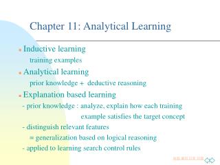
Analytical Learning
510 likes | 1.26k Views
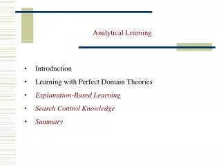
Analytical Learning. Introduction Learning with Perfect Domain Theories Explanation-Based Learning Search Control Knowledge Summary. Introduction. Learning algorithms like neural networks, decision trees, inductive logic programming, etc. all require a good number of examples to

Analytical Learning
E N D
Presentation Transcript
Analytical Learning • Introduction • Learning with Perfect Domain Theories • Explanation-Based Learning • Search Control Knowledge • Summary
Introduction Learning algorithms like neural networks, decision trees, inductive logic programming, etc. all require a good number of examples to be able to do good predictions. Learning Algorithm hypothesis dataset Dataset must be sufficiently large
Introduction We don’t need a large dataset if besides taking examples as input, the learning algorithm can take prior knowledge. Learning Algorithm hypothesis dataset Prior knowledge Dataset does not need to be large
Introduction Explanation-based learning uses prior knowledge to reduce the size of the hypothesis space. It analyzes each example to infer which features are relevant and which ones are irrelevant. Prior knowledge Hypothesis Space HS Reduced HS
Example Learning to Play Chess Suppose we want to learn a concept like “what is a board position in which black will lose the queen in x moves?”. Chess is a complex game. Each piece can occupy many positions. We would need many examples to learn this concept. But humans can learn these type of concepts with very few examples. Why?
Example Humans can analyze an example and use prior knowledge related to legal moves. From there it can generalize with only few examples. Example: why is this a positive example? “Because the white king is attacking both king and queen; black must avoid check, letting white capture the queen” reasoning
Example • What is the prior knowledge involved in playing chess? • It is knowledge about the rules of chess: • Legal moves for the knight and other pieces. • Players alternate moves in games. • To win you must capture the opponent’s king.
Inductive and Analytical Learning Inductive Learning Analytical Learning Input: HS, D, Input: HS, D, B Output: hypothesis h Output: h h is consistent with D h is consistent with D and B ( ~h --| B ) HS: Hypothesis Space D: Training Set B: Background knowledge
Example Analytical Learning • Input: • Dataset where each instance is a pair of objects represented • by the following predicates: Color, Volume, Owner, Material, • Density, On. Example: • On(Obj1,Obj2) Owner(Obj1,Fred) • Type(Obj1,Box) Owner(Obj2,Louise) • Type(Obj2,Endtable) Density(Obj1,0.3) • Color(Obj1,Red) Material(Obj1,Cardboard) • Color(Obj2,Blue) Material(Obj2,Wood) • Volume(Obj1,2)
Example Analytical Learning Hypothesis space: set of Horn clause rules. The head of each rule has the predicate SafeToStack. Example: SafeToStack(x,y) Volume(x,vx) ^ Volume(y,vy) ^ LassThan(vx,vy) Domain Theory: SafeToStack(x,y) ~Fragile(y) SafeToStack(x,y) Lighter(x,y) Lighter(x,y) Weight(x,wx) ^ Weight(y,wy) ^ LessThan(wx,wy)
Example Analytical Learning • Domain Theory: • SafeToStack(x,y) ~Fragile(y) • SafeToStack(x,y) Lighter(x,y) • Lighter(x,y) Weight(x,wx) ^ Weight(y,wy) ^ LessThan(wx,wy) • … • Fragile(x) Material(x,Glass) • Note: • The domain theory refers to predicates not contained • in the examples. • The domain theory is sufficient to prove the example is true.
Perfect Domain Theories A domain theory is correct if each statement is true. A domain theory is complete if it covers every positive example of the instance space (w.r.t a target concept and instance space). A perfect domain theory is correct and complete.
Perfect Domain Theories Examples of where to find perfect domain theories: Rules of chess Examples of where not to find perfect domain theories: SafetoStack problem We will look into learning problems with perfect domain theories only.
Explanation Based Learning Algorithm • We consider an algorithm that has the following properties: • It is a sequential covering algorithm considering the data incrementally • For each positive example not covered by the current rules it forms a new rule by: • Explaining the new positive example. • Analyzing the explanation to find a generalization. • Refining the current hypothesis by adding a new • Horn Clause rule to cover the example.
Explanation Based Learning Algorithm • Prolog-EBG (Kedar-Cabelli and McCarty 87). • LearnedRules {} • Pos Positive examples from training examples • For each positive example X in Pos not covered • by LearnedRules do • Explain • Use the domain theory to explain that X • satisfies the target.
Explanation Based Learning Algorithm • Prolog-EBG (Kedar-Cabelli and McCarty 87). • b. Analyze • Find the most general set of features of X sufficient • to satisfy the target according to the explanation. • Refine • LearnedRules += NewHornClause • NewHornClause: Target sufficient features • 4. Return LearnedRules
Explaining the Example • For each positive example X in Pos not covered by • LearnedRules do • Explain • Use the domain theory to explain that X satisfies • the target concept.
Explaining the Example The explanation is a proof that the example belongs to the target (if the theory is perfect): On(Obj1,Obj2) Owner(Obj1,Fred) Type(Obj1,Box) Owner(Obj2,Louise) Type(Obj2,Endtable) Density(Obj1,0.3) Color(Obj1,Red) Material(Obj1,Cardboard) Color(Obj2,Blue) Material(Obj2,Wood) Volume(Obj1,2)
Explanation SafeToStack(Obj1,Obj2) Lighter(Obj1,Obj2) Weight(Obj1,0.6) Weight(Obj2,5) LessThan(0.6,5) Volume(Obj1,2) Density(Obj1,0.3) Equal(0.6,2*0.3) Type(Obj2,Endtable)
Explanation • Considerations: • There might be more than one explanation to the example. In that case one or all explanations may be used. • An explanation is obtained using a backward chaining search as is done by Prolog. Prolog-EBG stops when it finds the first proof.
Analyze Many features appear in an example. Of them, how many are truly relevant? We consider as relevant those features that show in the explanation. Example: Relevant feature: Density Irrelevant feature: Owner
Analyze Taking the leaves of the explanation and substituting variables x and y for Obj1, and Obj2: SafeToStack(x,y) Volume(x,2) ^ Density(x,0.3) ^ Type(y,Endtable)
Analyze • Considerations: • We omit features independent of x and y such as Equal(0.6,times(2,0.3)) and LessThan(0.6,5). • The rule is now more general and can serve to explain other instances matching the rule. • A more general form of generalization called regression finds the most general rule explaining the example.
Refine • The current hypothesis is the set of Horn clauses that we have constructed up to this point. • Using sequential covering we keep adding more rules, thus refining our hypothesis. • A new instance is negative if it is not covered by any rule.
Remarks • Explanation Based Learning (EBL) justifies the hypothesis by using prior knowledge. • The explanation or proof shows which features are relevant. • Each Horn clause is a sufficient condition for satisfying the target concept.
Remarks • The success of the method depends on how the domain theory is formulated. • We assumed the theory is correct and complete. If this is not the case the learned concept may be incorrect.