Download
1 / 55
550 likes | 694 Views
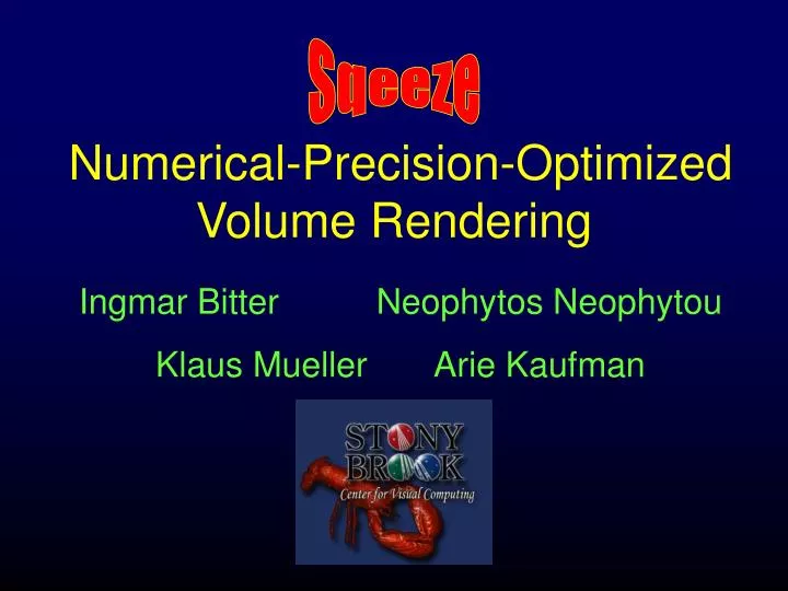
Sqeeze. Numerical-Precision-Optimized Volume Rendering. Ingmar Bitter Neophytos Neophytou Klaus Mueller Arie Kaufman. Sqeeze. Numerical-Precision-Optimized Volume Rendering. Ingmar Bitter Neophytos Neophytou Klaus Mueller Arie Kaufman. Outline.

E N D
Sqeeze Numerical-Precision-Optimized Volume Rendering Ingmar Bitter Neophytos Neophytou Klaus Mueller Arie Kaufman
Sqeeze Numerical-Precision-Optimized Volume Rendering Ingmar Bitter Neophytos Neophytou Klaus Mueller Arie Kaufman
Outline • Numerical precision - a rendering resource
Outline • Numerical precision - a rendering resource • Fixed-point arithmetic
Outline • Numerical precision - a rendering resource • Fixed-point arithmetic • Reverse order precision analysis • Compositing, shading, gradients, classification, sampling/splatting, sample/splat location
Outline • Numerical precision - a rendering resource • Fixed-point arithmetic • Reverse order precision analysis • Compositing, shading, gradients, classification,sampling/splatting, sample/splat location • Results
Outline • Numerical precision - a rendering resource • Fixed-point arithmetic • Reverse order precision analysis • Compositing, shading, gradients, classification, sampling/splatting, sample/splat location • Results • Conclusions
Numerical Precision: A Resource • Double precision computation for all – ideal?
Numerical Precision: A Resource • Double precision computation for all – ideal? • slower then all other alternatives • not possible on graphics cards (at least for now) • expensive on custom chip implementations • and most importantly: not needed to create best possible images!!
Numerical Precision: A Resource • Double precision computation for all – ideal? • slower then all other alternatives • not possible on graphics cards (at least for now) • expensive on custom chip implementations • and most importantly: not needed to create best possible images!! reasons: predominantly 8-bit displays (per channel) limited range intervals throughout
Current Status • Stable volume rendering pipeline: both CPU and GPU[LL94, Lev88, MJC02, Wes90, EKE01, RSEB00] • Interpolation before classification, even for splatting [MMC99] • Caching optimized for volume rendering[Kni00, LCCK02, PSL98] • Precision-limited rendering systems: ATI, NVidia,VolumePro [PHK99], VizardII [MKW02], UltraVis [Kni00] • Completely fixed: final output image display bit precision • 8 bits per RGB color channel on CRTs and LCDs • 8 bits max in DVI standard • SGIs 12 bit color displays are nearly extinct • Radiologists’ requirements are not mass market, same analysis applies
OpenGL Arithmetic: 12=1? • Representation [0, 255] a = b = 255 • Computation = a[0, 255]×b[0, 255] >> 8; = 254 wrong 1 mult, one shift • Alternatively: tmp = a[0, 255]×b[0, 255] + 128; result = (tmp+(tmp >> 8)) >> 8; = 255, correct [Bli95] 1 mult, 2 adds, 2 shifts
OpenGL Arithmetic: 12=1? • Representation: fixed-point I.Fb • I.Fb = I integer bits, F fraction bits • 8 bits 1.7b fixed point number then a = b = 11.7b = 128 • Computation = a1.7b× b1.7b >> 7 = 128 correct 1 mult, one shift one fewer bit of resolution, but OK (we will see)
Reverse Order Precision Analysis Ray Casting Splatting • Unified ray casting and splatting pipelines • Composite creates the final image Sample Location Splat Location Sample Splat Classify Gradient Shade Composite
Reverse Order Precision Analysis Ray Casting Splatting • Unified ray casting and splatting pipelines • Composite creates the final image • Precisionrequirements propagate backwards Sample Location Splat Location Sample Splat Classify Gradient Shade Composite
Compositing - Math • Pre-(alpha)-multiplied colors: • C = αC = αR, αG, αB • Alpha correction (r samples per unit): • Tcorrected = (1- α)r
Compositing - Math • Pre-(alpha)-multiplied colors: • C = αC = αR, αG, αB • Alpha correction: • Tcorrected = (1- α)r • With back-to-front compositing: • CCompositingBuffer×= Tcorrected += Cfront • TCompositingBuffer×= Tcorrected; αCompositingBuffer= 1-Tcorrected • perform multiplication N timesper pixel correct solution needs N× F × r bits precision T/CCompositingBuffer • Tcorrected, Cfront T/CCompositingBuffer
Compositing – Precision Theory • 8-bit destination resolution • therefore all partial results can be rounded • drop all bits not contributing to the 8 most significant bits (MSB) • Adding N = 2p samples • allows 8+p bits to influence the 8 MSB • Conversion from αCompositingBufferC to C for display (division) • allows 8+p more bits to influence the 8 MSB • Conversion from αcorrectedC to C for display • allows r times as many bits to influence the 8 MSB • Sufficient resolution is: r× 2 × (8+p) for C, r× (8+p) for α • 32/16 bits for C/αCompositingBuffer for 2563 volumes and no super-sampling • 608 bits for 5122×2048 volumes and 16 samples per voxel
Compositing – Precision Theory • 8-bit destination resolution • therefore all partial results can be rounded • drop all bits not contributing to the 8 most significant bits (MSB) • Adding N = 2p samples • allows 8+p bits to influence the 8 MSB • Conversion from αCompositingBufferC to C for display (division) • allows 8+p more bits to influence the 8 MSB • Conversion from αcorrectedC to C for display • allows r times as many bits to influence the 8 MSB • Sufficient resolution is: r× 2 × (8+p) for C, r× (8+p) for α • 32/16 bits for C/αCompositingBuffer for 2563 volumes and no super-sampling • 608 bits for 5122×2048 volumes and 16 samples per voxel
Compositing – Precision Theory • 8-bit destination resolution • therefore all partial results can be rounded • drop all bits not contributing to the 8 most significant bits (MSB) • Adding N = 2p samples • allows 8+p bits to influence the 8 MSB • Conversion from αCompositingBufferC to C for display (division) • allows 8+p more bits to influence the 8 MSB • Conversion from αcorrectedC to C for display • allows r times as many bits to influence the 8 MSB • Sufficient resolution is: r× 2 × (8+p) for C, r× (8+p) for α • 32/16 bits for C/αCompositingBuffer for 2563 volumes and no super-sampling • 608 bits for 5122×2048 volumes and 16 samples per voxel
Compositing – Precision Theory • 8-bit destination resolution • therefore all partial results can be rounded • drop all bits not contributing to the 8 most significant bits (MSB) • Adding N = 2p samples • allows 8+p bits to influence the 8 MSB • Conversion from αCompositingBufferC to C for display (division) • allows 8+p more bits to influence the 8 MSB • Conversion from αcorrectedC to C for display • allows r times as many bits to influence the 8 MSB • Sufficient resolution is: r× 2 × (8+p) for C, r× (8+p) for α • 32/16 bits for C/αCompositingBuffer for 2563 volumes and no super-sampling • 608 bits for 5122×2048 volumes and 16 samples per voxel
Compositing – Precision Theory • 8-bit destination resolution • therefore all partial results can be rounded • drop all bits not contributing to the 8 most significant bits (MSB) • Adding N = 2p samples • allows 8+p bits to influence the 8 MSB • Conversion from αCompositingBufferC to C for display (division) • allows 8+p more bits to influence the 8 MSB • Conversion from αcorrectedC to C for display • allows r times as many bits to influence the 8 MSB • Sufficient resolution is: r× 2 × (8+p) for C, r× (8+p) for α • 32/16 bits for C/αCompositingBuffer for 2563 volumes and no super-sampling • 608 bits for 5122×2048 volumes and 16 samples per voxel
Compositing – Precision Practice • No alpha correction (r = 1): 2 × (8+p) bits • Iso-surface rendering using “old fashioned” OpenGL: • store not αC but C in frame buffer: (8+p) • bright colors: 5+p • at most 8 non-zero samples per ray (p=3): 5+3=8 bits standard 24 bit RGBA frame buffer is adequate • Fog visualization • what matters is the ability to see objects though volumetric fog (substance with low opacity) • visual experiments show 15 fractional bits are sufficient
Compositing – Precision Practice • No alpha correction (r = 1): 2 × (8+p) bits • Iso-surface rendering using “old fashioned” OpenGL: • store not αC but C in frame buffer: (8+p) • bright colors: 5+p • at most 8 non-zero samples per ray (p=3): 5+3=8 bits standard 24 bit RGBA frame buffer is adequate • Fog visualization • what matters is the ability to see objects though volumetric fog (substance with low opacity) • visual experiments show 15 fractional bits are sufficient
Compositing – Precision Practice • No alpha correction (r = 1): 2 × (8+p) bits • Iso-surface rendering using “old fashioned” OpenGL: • store not αC but C in frame buffer: (8+p) • bright colors: 5+p • at most 8 non-zero samples per ray (p=3): 5+3=8 bits standard 24 bit RGBA frame buffer is adequate • Fog visualization • what matters is the ability to see objects though volumetric fog (substance with low opacity) • visual experiments show 15 fractional bits are sufficient
Compositing – Precision Practice • No alpha correction (r = 1): 2 × (8+p) bits • Iso-surface rendering using “old fashioned” OpenGL: • store not αC but C in frame buffer: (8+p) • bright colors: 5+p • at most 8 non-zero samples per ray (p=3): 5+3=8 bits standard 24 bit RGBA frame buffer is adequate • Fog visualization • what matters is the ability to see objects though volumetric fog (substance with low opacity) • visual experiments show 15 fractional bits are sufficient
Compositing – Precision Practice • No alpha correction (r = 1): 2 × (8+p) bits • Iso-surface rendering using “old fashioned” OpenGL: • store not αC but C in frame buffer: (8+p) • bright colors: 5+p • at most 8 non-zero samples per ray (p=3): 5+3=8 bits standard 24 bit RGBA frame buffer is adequate • Fog visualization • what matters is the ability to see objects though volumetric fog (substance with low opacity) • visual experiments show 15 fractional bits are sufficient
Compositing – Precision Practice • No alpha correction (r = 1): 2 × (8+p) bits • Iso-surface rendering using “old fashioned” OpenGL: • store not αC but C in frame buffer: (8+p) • bright colors: 5+p • at most 8 non-zero samples per ray (p=3): 5+3=8 bits standard 24 bit RGBA frame buffer is adequate • Fog visualization • what matters is the ability to see objects though volumetric fog (substance with low opacity) • visual experiments show 15 fractional bits are sufficient
Compositing – Conclusion Least-significant-bit-fog at various bit precisions 8 10 12 14 15 16 5123dataset r = 2 • Preferred bit-aware back-to-front compositing equations: • αC1.15b×= T1.15bsample += C1.15bsample • T1.15b×= T1.15bsample
Shading - Math • PhongCcolor = kambient OobjectColor IlightIntensity+kdiffuse O Σi{ Ii (N•Li) } +kspecular Σi{ Ii (R•Li)r } • k є [0,1] kambient +kdiffuse +kspecular =1 • OobjectColor (8 bit) and IlightIntensityє [0,1] • N•Li andR•Li є [-1,1], but є [0,1] after clamping • PhongCcolor = є [0,1] (possibly clamping Σi)
Shading - Analysis • PhongCcolor needs to be as precise as 1.15b • Use 16.16b for all multiplications [0,1)× [0,1] • sufficient precision and no overflow
Shading – New Computation • Replace specular exponentiation with recursive multiplies • repeatedly multiply number with itself • works for all exponents r=2n • when r=26 (16 bit precision), then max error < 0.005% • better results than Knittel’s parabola approximation
Shading – New Computation • Replace specular exponentiation with recursive multiplies • repeatedly multiply number with itself • works for all exponents r=2n • when r=26 (16 bit precision), then max error < 0.005% • better results than Knittel’s parabola approximation Knittel’s parabola pow r=2n
Shading - Conclusion • Preferred bit-aware Phong shading equation: C16.16b = k16.16bambient O0.8bobjectColor I16.16blight+k16.16bdiffuseO0.8bΣi{ I16.16bi (N16.16b•L16.16bi) } +k16.16bspecular Σi{ I16.16bi (R16.16b•L16.16bi)2^n }
Gradients - Math • Gx = 0.5 sample(x+1,y,z) -0.5 sample(x-1,y,z) • Gy = 0.5 sample(x,y+1,z) -0.5 sample(x,y-1,z) • Gy = 0.5 sample(x,y,z+1) -0.5 sample(x,y,z-1)
Gradients - Analysis • G = G1.Fb • Discrete nearest gradient vector neighbors • sin φ = 1/2F,sin φ ≈ φ → φ ≈ 1/2F • Maximum error for specular intensity, large r • r = 64, 164 != 1, but 164 = (1- 1/2F)64 • error of 22%, 6.1%, 1.6%, 0.4%for F of 8, 10, 12, 14 φ
Gradients - Analysis • 5123-sized spheres with Phong highlights • 4, 6, 8, 10, 12, 14 bit gradients • Diffuse artifacts for 4 and 6 bits • Specular artifacts up to 10 bits 4 6 8 10 12 14 10 12 14
Gradients - Conclusion • Thus, 12 bits dynamic range is needed • Now consider normalization: • reduces I.Fb to 1.Fb • up to I bits will be added to the fractional part • Volume samples often have 12 bits • Gx,y,z with 12.12b minimum representation • Gx,y,z with 16.16b preferred representation • leaves room for interpolation bits in normalization
Classification – Prelims and Recaps • Use of T instead of α is more efficient in compositing operation • Largest visual precision/quantization error occurs at high transparencies (low opacities) • need more bits for T than for C, just to be sure • Want transfer function lookup table to be cache-friendly • power-of-2 RGBA-tuple alignment • Would like to use pre-integrated classification for color and opacity transfer functions [EKE01, MGS02]
Classification – Prelims and Recaps • Use of T instead of α is more efficient in compositing operation • Largest visual precision/quantization error occurs at high transparencies (low opacities) • need more bits for T than for C, just to be sure • Want transfer function lookup table to be cache-friendly • power-of-2 RGBA-tuple alignment • Would like to use pre-integrated classification for color and opacity transfer functions [EKE01, MGS02]
Classification – Prelims and Recaps • Use of T instead of α is more efficient in compositing operation • Largest visual precision/quantization error occurs at high transparencies (low opacities) • need more bits for T than for C, just to be sure • Want transfer function lookup table to be cache-friendly • power-of-2 RGBA-tuple alignment • Would like to use pre-integrated classification for color and opacity transfer functions [EKE01, MGS02]
Classification – Prelims and Recaps • Use of T instead of α is more efficient in compositing operation • Largest visual precision/quantization error occurs at high transparencies (low opacities) • need more bits for T than for C, just to be sure • Want transfer function lookup table to be cache-friendly • power-of-2 RGBA-tuple alignment • Would like to use pre-integrated classification for color and opacity transfer functions[EKE01, MGS02]
Classification - Math • Desired lookup table entries: R1.8bG1.8bB1.8bT1.16b 5.5 bytes • Common lookup table entries: R0.8bG0.8bB0.8bα0.8b 4 bytes
Classification - Math • Desired lookup table entries: R1.8bG1.8bB1.8bT1.16b 5.5 bytes • Common lookup table entries: R0.8bG0.8bB0.8bα0.8b 4 bytes • Better lookup table entries: R0.8bG0.8bB0.8bsqrt(α)0.8b spreads low α • Computed lookup after T = 1-(sqrt(α)2): R0.8bG0.8bB0.8bT1.16b squaring doubles precision
Classification - Conclusion Foot with least-significant-thin-tissue-fog • Preferred bit-aware lookup table entries: R0.8bG0.8bB0.8bsqrt(α)0.8b α0.8b sqrt(α)0.8b α0.16b
Sample Interpolation - Math • sample = voxel0× (1-w) + voxel1× w • sample = w × (voxel1 - voxel0) + voxel0 • Requirements: • Gx,y,z, derived from samples,need 12 bit dynamic range • samples need 12 bit values for transfer function lookup • cover both low and high dynamic range neighborhoods • Therefore, sample12.12b is a minimum requirement • integer part comes from voxels voxel12.0b • fractional part comes from interpolation w1.12b
Sample Interpolation - Conclusion • Preferred bit-aware sample interpolation: sample12.12b = w1.12b× (voxel112.0b - voxel012.0b) + voxel012.0b • Splats start on voxels, need no interpolation: splat12.0b = voxel12.0b
Sample Location - Math k • k-th sample location = startPos + Σk Vinc • Perspective rays need to differ enough to allow 1024 rays across 60 degrees, or 0.05◦ • sin φ = (k 1/2F) / k,sin φ ≈ φ → φ ≈ 1/2F • F = 6, 12, 16 → φ = 0.9◦, 0.05◦, 0.0009◦ • Also, need to address 2048 slices (integer positions) → 11bits • Thus, need overall 11.12b φ
Sample Location - Conclusion • Preferred bit-aware sample location: • perspective projection: sampleLocation11.12b = startPos11.12b + Σ Vinc1.12b • parallel projection: sampleLocation11.6b (0.9◦ OK)
Splat Scan Conversion - Math • Splats project onto image grid → reverse rays • Allow as many as 2048 splat rays across 60 degrees, or 0.025◦ • Hence, twice the ray casting precision • one extra fractional bit F=13 • Also address 2048 slices (11bits) • Thus, need overall 11.13b φ