Download
1 / 193
1.93k likes | 1.94k Views
RNA-Seq Workshop for the Bioinformatician. University of Pennsylvania November 6, 2014. Gregory R. Grant (ggrant@pcbi.upenn.edu). http://bioinf.itmat.upenn.edu/workshop/upenn-workshop_11-6-14.ppt. ITMAT Bioinformatics. Gregory Grant Eun Ji Kim Katharina Hayer Faith Coldren

E N D
RNA-Seq Workshop for the Bioinformatician University of Pennsylvania November 6, 2014 Gregory R. Grant (ggrant@pcbi.upenn.edu) http://bioinf.itmat.upenn.edu/workshop/upenn-workshop_11-6-14.ppt
ITMAT Bioinformatics • Gregory Grant • EunJi Kim • Katharina Hayer • Faith Coldren • Dimitra Sarantopoulou • Nicholas Lahens • Anand Srinivasan
Choosing the Right Method • A large percent of RNA-Seq users are after evident effects. • Large fold change of well expressed genes • Well annotated genes • Uncomplicated question • Direct comparison between two experimental conditions. • You can usually find such effects no matter how you look for them. • Use the simplest and cheapest computational methods available. • Most of the time microarrays are still sufficient for this purpose.
RNA-Seq Data • Full length mRNA cannot (yet) be sequenced accurately and cheaply. • Instead typically RNA are fragmented into fragments between 100 and 500 bases. • Then small segments of ~100 bases are sequenced from one or both ends of the fragments.
Data are Quantitative • Reads are aligned to the genome. • Data are represented as “depth of coverage” plots. • The higher a gene is expressed, the more reads we find for that gene. • The higher the peak, the greater the gene is expressed.
Part 1 • Generalities • Pipeline-birds-eye view • System requirements • Study Design • Fastq • Alignment • Visualizing alignments
Generalities • High throughput sequencing is still in its infancy. • All aspects of analysis are under active development. • Every study is a special case. • Push-button approaches can be hazardous. • Even the most standard methods, that are widely used, are cumbersome to run. • Data sets are enormous • Their sheer size alone presents difficult computational issues. • To get the most out of the data you will have to chaperone them by hand every step of the pipeline. • With continuous reality-checking.
Generalities (continued) • Today we will look at the main issues that arise with RNA-Seq data analysis. • We will look at what works and what doesn’t work. • A good analysis requires constant vigilance. • Make integrity checking an obsessive habit. • Mental reality checks • Systematic assessments. • This business is not for the faint of heart.
The Landscape of Sequencing Platforms Illumina Stock Price • A couple years ago there were five or six serious contenders. • Solid • 454 • Illumina • Heliscope • Ion Torrent • At this point Illumina has 99% of the market. • The only serious contender left is Life Technology’s Ion Torrent. • Therefore, we will focus entirely on the analysis of Illumina data.
RNA-Seq Analysis- the main steps - Raw Data Alignment Normalization Quantification Statistical Analysis Data Management and Deployment
The RNA-Seq Analysis Pipeline • The main analysis steps we will address today are: Alignment Normalization QuantificationDifferential Expression • Our Philosophy: • Benchmark the tools being made available by the community. • Build our own tools only when absolutely necessary. • Everybody is trying to build toolsand to win the popularity contest. • BUT • Benchmarking provided by the tool builders is usually biased. • As the target audience for these tools we need thorough and objective benchmarking. • For lack of time and resources, most users buy into the hype and proceed on faith - with perilous outcomes. • Using objective and unbiased benchmarking we will see that some of the most popular algorithms dramatically underperform other less known methods. • In short: Benchmarking is necessary.
The complex landscape of published analysis methods. • Don’t try to read this - the point is that there are dozens of available apps for every step of the pipeline. Figure from Alamancos et al., 2014, http://arxiv.org/abs/1304.5952
System Requirements • Unless you are working with one or very few samples, you will need access to some sort of cluster computing environment. • Today we will use Upenn’s brand new PMACS cluster. • Each node on the cluster should have at least 8 Gb of RAM • We will consider some algorithms that require upwards of 30 Gb of RAM to run • Be prepared to spend hundreds of dollars on compute time to analyze one study. • If there are dozens of replicates this can rise to four digits • Budget for this in your grants
More Requirements • Files are enormous • One sample of 100 million read pairs can take up 300-400 Gb of disk space to analyze. • A study with 20 samples or more will require Terabytes of disk space. • Analysis require a lot of I/O. • The file system needs to be fast. • A Tb of files may have to be read and written dozens of times to get a full study through an analysis pipeline.
Cloud Computing • If your institution does not have the necessary compute resources, then you can always check them out by the hour at aws.amazon.com. • Google also wants your business, but they are lagging way behind Amazon. • Amazon has very large, and growing, farms of computers that are available for instant access. • The interface is somewhat complicated. • A subject that deserves its own workshop.
More Requirements • Fast public html web server. • Must be able to serve large files (hundreds of megabytes). • To display large tracks of data in the genome browser, you store them in your own public html space and point the genome browser to them. • The maximum sized file you can upload directly is somewhere between 50 and 100 Mb. • If you do not have such a public html server, then you can always use buckets at http://aws.amazon.com.
Duration of Analysis If you run into complications, be prepared for it to take several weeks or longer to perform a good analysis. • And things always seem to get complicated. • It’s almost impossible to give reliable ETAs. • What seems like the easiest step can surprise you. • There is a daunting amount of information in an RNA-Seq data set. • Start simple and dig deeper into things only if necessary
Text • We work mainly with text files. • We edit “small” files with Emacs or vi. • Emacs will typically open a file up to 250 Mb in size. • For larger files you will have to write scripts to edit them. • Line editors such as Ed, Sed and Awk are useful. • Not essential, but they can help. • There’s nothing you can’t do with a little bit of Perl, Python or Ruby.
Tab Delimited Text • The text files are often tab delimited. • Sometimes we export tab delimited text from Excel. • When you do this they may have different newline characters than UNIX understands. • Use “cat –v <file> | more” to check for strange characters at the end of lines. Something like this: > cat –v file.txt | more The rain in spainfalls^M mainly in the plain.^M • Push text files from Excel through dos2unix to change to unix-friendly newline characters.
Useful Unix Commands for Tab Delimited Text • cut –f n <file> • n can be an integer or spans of integers or combinations separated by commas Or more generally: • awk '{print $1, $2, $1, $3}' <file> Or split on spaces instead of tabs: • awk –F“ ” '{print $1, $2, $1, $3} ' <file> • paste <file1> <file2> • less –S Or the following which will align columns nicely: • column -s$'\t' -t <file> | less -S
Scripts • It won’t be possible to perform an effective RNA-Seq analysis without being able to write scripts. • At least at the basic level. • Perl and Python are widely used in the field. • Know your RegExp’s. • There are also packages of tools: • SAM tools • Picard tools • Galaxy • But they never do everything you need to do.
Scripting and Efficiency • Any operation you apply to an entire file of RNA-Seq data will require significant time to run. • And may require considerable RAM. • Even the most basic information from all reads cannot be stored in RAM all at once. • Just storing the read ID from 100 Million reads, assuming each takes 100 Bytes, adds up to 10 Gigabyte of RAM. • Perl/Python are not very efficient with how they allocate memory for data structures. • Therefore, most tasks must be split up and processed in pieces. • Parallelization is key. • It’s not unusual to use 100 to 200 compute cores while running the pipeline.
Myths • RNA-Seq overcomes every issue inherent in microarrays. • Data are so replicable that we no longer have to worry about technical confounders. • E.g. date, tech, machine, etc.. • Data are so clean that replication is no longer necessary. • Data are so perfect that we no longer have to worry about normalization.
So What is Better About RNA-Seq? • The dynamic range. • Microarrays • high background • low saturation point • RNA-Seq • Zero to infinity. • We can finally conclude when genes are not expressed with some reasonable degree of reliability.
So What is Better About RNA-Seq? • Coverage. • Microarrays • One, or at most a few probes per gene. • RNA-Seq • Signal at every single base. • Signal from novel features and junctions.
So What is Better About RNA-Seq? • Assessment of fold change. • Microarrays: Impossible. • Microarray measurements are on arbitrary scale. • The guy down the hall may have the same values as you but with 100 added to each intensity. • His fold changes will be lower than yours. • RNA-Seq: Possible. • The read counts divided by the total number of reads gives an estimate of the proportion of that gene in a sample. • Assuming any technical bias is the same in all samples and so cancels itself out. • Much more on this later. • Okay, this may be a little optimistic. But there’s a chance, while in microarrays it is certainly meaningless.
Decisions • You cannot properly sequence all types of RNA at the same time. • Coding versus Non-Coding RNA • Fragment size for coding: 200-400 bases • This would miss short non-coding RNAs • Read lengths. • Standard is now 100 bases, and growing. • The longer the read, the more costly, but the more likely it is to align it uniquely to the genome. • Single-end or Paired-end. • We obviously get a lot more information from paired-end. • Strand Specific versus Non-Strand Specific. • Ribosomal depletion protocol. • Ribo zero • PolyA selection • Depth of coverage.
How Deep to Sequence? • At around 80 million fragments we start to see diminished returns.
Depth versus Reps • You are usually better off with eight (biological) replicates at 40 million reads than four with 80 million. • One lane on the current machines produces hundreds of millions of read (pairs). • This is usually overkill for one sample. • Consider multiplexing. • With “barcodes” you can put many samples in one lane. • But, take into consideration the purity of your sample. • If the cell type of interest is only 10% of your sample, then you will need significantly deeper coverage to get at what’s going on in those cells.
Study Design Issues • RNA-Seq minimizes some of the technical variability that microarrays suffer from. • But no data type can reduce biological variability. • In fact given the greater number of features measured by RNA-Seq, the downstream statistics may require more replicates than microarrays to achieve the same power. • We found, in a typical data set, that we cannot detect anything less than 2-fold with less than five replicates.
How Many Replicates? • How many replicates to do depends on the inherent variability of the population and the effect size you are looking for. • Classical power analyses are not applicable • Multiple testing • Different genes have different distributions • There is no feasible pilot study or reliable simulation to this end • Therefore we do as many replicates as we can • We have done as many as eight replicates per group
Randomization • Full randomization is necessary at every stage. • Sample procurement. • Sample preparation. • Sequencing. • “Randomization” means if you have WT and Mutant, never do anything where all WT are processed as one batch and all Mutant are processed as a separate batch. • Alternate conditions in every step. • Alternate samples on the flow cell. • Multiplexing can facilitate randomization • Meticulously record information about every step: • Who did it. • When they did it. • How they did it. • Even the gender of the experimenter is known to make a difference.
File Format #1: FastA • Most of you are probably familiar with fastA format for text files of sequences. • Each sequence has a name line that starts with “>”, followed by some number of lines of sequence. > seq1 CGTACTACGATCGTATACGATCGAGCTA TACGTCGGCGTTATAAATGCGTATGTGT > seq2 TGATGCGTATCGATGCTATGAGCTATTT TGGTTATCCATACCGATAGTACGCGATT
File Format #2: FastQ • Data coming off the sequencing machines come in FastQ format. • Each read has four lines. E.g.: • @HWI-ST423:253:C0HP8ACXX:1:1201:6247:13708 2:N:0:AGTTCC • CCCGGACTGGGCACAGGGTGGGCAAGCGCGTGGAGGTTGCTGGCGGAGTGGC…. • + • CCCFFFFFHHHHGJGGGIAFDGGIGHGIGJAHIEHH;DHHFHFFD',8(<?@B&5:65.... • Line 1 is the read ID. • This contains information such as tile, barcode, etc... • Line 2 is the actual read sequence. • This may contain missing values encoded as “N”.
Line 3 is usually simply a plus sign. • Line 4 gives a quality scores for each base. • This quality score encoding keeps changing, the latest is a score from 0 to 41 encoded by a range of ascii characters: • !"#$%&'()*+,-./0123456789:;<=>?@ABCDEFGHIJ • Therefore “J” are highest quality bases and “!” are the lowest. • Quality is typically low for the first hundred reads, give or take. • Quality also tends to decrease at the ends of the read.
FastQ Continued • If the data are paired-end then the data will come as twoFastQ files. • One with the forward reads and one with the reverse. • They are in the same order in the two files, so pairing forward/reverse reads is easy. • If the data are strand specific then: • If the forward read maps to the positive strand, then the fragment actually sequenced came from the positive strand. • If the forward read maps to the reverse strand, then the fragment actually sequenced came from the reverse strand. • Although sometimes it is the other way around. • BLATing a few reads in the genome browser will tell you which way it goes…
Alignment • Alignment is the first step in the pipeline. • We always align to the genome. • And possibly also to the transcriptome. • Gene annotation is not complete enough for any species to rely solely on the transcriptome. • Much of the data comes from introns or intergenic regions. • Transcription is complicated and not well understood. • Paired-end reads should align consistent to being opposite ends of a short fragment. • Three possibilities: • Read (pair) aligns uniquely. • Called a unique mapper. • Read (pair) aligns to multiple locations. • Called a multi-mapper or a non-unique mapper. • Read (pair) does not align. • Called a non-mapper.
Visualizing the Alignment- Genome Browsers - • The UCSC genome browser is a powerful and flexible way to view RNA-Seq data. http://genome.ucsc.edu/ • The UCSC genome browser allows you to upload your own tracks and save and share your sessions. • It doesn’t allow read level visualization yet. • There are a number of genome browsers each with their own advantages. • Some run locally and some run remotely. • E.g. The UCSC browser can be installed locally • Some allow you to zoom in to see individual read alignments. • E.g. IGV from the Broad institute.
The UCSC Genome Browser • RNA-Seq “coverage plot” (in red). • Gene models (in blue) (three transcripts shown) . • Note the intron and intergenic signal.
Coverage and Junction Tracks • Junctions are shown. • Bluejunctions are annotated. • Greenare inferred from the data but not annotated. • Junctions come with a quantification. • In the form of counts of reads which span the gap.
Replicabilityof Signal • These two samples were done a year apart on independent animals. • Even the local variability and intron signal is remarkably consistent.
Browse • Take some time to browse some real data to build your intuition. • Intuition is your best integrity check. • Learn to recognize what is normal and what is unusual. • The following few slides show some real data • Some normal behavior • Some strange but not infrequent behavior.
Zooming in on one gene- a simple case - • This is what we like to see. • One splice form, fairly uniform coverage, all junctions represented. • If all genes were like this, life would be easy.
Mostgenes arelike this • Exons are small. • Except for the 3’ exon (the last one) which is usually much larger. • Introns are much bigger than exons. • 3’ UTRs are large. 5’ UTRs are small. • UTR = “Un-Translated Region”.
A slightly more complicated example • What is that orphaned signal on the left? • Is the annotation wrong and that is actually another exon?
Look at the Junctions • No junctions connect to that signal on the left. • So it’s probably not part of the same gene.
Turn on another annotation track • Turning on ENSEMBL it appears to be a small one-exon gene. • ENSEMBL is generally more liberal than RefSeq. • But RefSeq does indicate two splice forms of the gene on the right, while ENSEMBL only one. • Take home message: there is no best annotation track.
Looking Closer • Zooming in on the gene, can we figure out what is really going on? • Are both annotated forms expressed? • There is at least one unannotated form expressed. • Green junction where exon 3 is skipped by 28 reads • Let’s zoom in on exon 2. exon 2 exon 3