Download
1 / 25
250 likes | 266 Views
Learn about Bayesian methods for data classification and segmentation, including measuring independence and dependency of attributes, and their applications in gene analysis, spam email filtering, and more.

E N D
Data Classification and Segmentation: Bayesian Methods III HK Book: Section 7.4, Domingos’ Paper (online) Instructor: Qiang Yang Hong Kong University of Science and Technology Qyang@cs.ust.hk Thanks: Dan Weld, Eibe Frank
Independence Test • Naïve Bayesian’s good performance may be due to independence of attributes? • Modeling independence of attributes Am and An • D() is zero when completely independent • D() is large if dependent
How to measure independence? • H(A|C): the once the class C is given, how much is A given? • In other words, how random is A once C is given • We know randomness can be measured in Entropy • Entropy is –p*log(p), and then summed over all possible values • Thus, to measure the dependence of A on C, we can look at each value Ci of C, such that under Ci, • Find the entropy of A • Then, sum over all possible Ci
Measuring dependency • Example: C=Play attribute, A=Windy Attribute • C1=yes, C2=no • Pr(C=Yes)=9/14 • When C=C1 (Play = yes) • A=True: 3 counts • A=False: 6 counts • Pr(A=True and C=C1)=3/14 • Pr(A=False and C=C1)=6/14 • When C=C2 (no) • Pr(A=True and C=C2)=3/14 • Pr(A=False and C=C2)=2/14 • H(A|C)=9/14*[(-3/14)log(3/14)-(6/14)log(6/14)]+5/14*[-3/14log(3/14)-2/14log(2/14)]
Property of H(A|C) • If A is completely dependent on C, what is H(A|C)? • In the extreme case, whenever C=yes, A is true; whenever C=no, A=false. • Pr(C=yes and A=true)=1 • Pr(C=yes and A=false)=0 • H(A|C)=? • The other extreme: if A is completely independent on C, what is H(A|C)? • Pr(…) between 0 and 1, • H(A|C)=??
Extending to two attributes • For A1 and A2, we simply consider the Cartesian product of their values • This gives a single attribute • Then we measure the dependency of A1A2 (a new attribute) on class C • Example: Consider A1=Humidity and A2=Windy, Class= Play • Humidity={high, normal} • Windy={True, False} • A1A2=HumidityWindy={hightrue, highfalse, normaltrue, normalfalse}
Putting them together • When the two attributes Am and An are independent, given C, • H(AmAn |C)=H(Am|C)+H(An|C) • D(…) = 0 • When they are dependent • D(…) is a large value • Thus, D (…) is a measure of dependency between attributes
Why Perform So well? (section 4 of paper) • Assume three attributes A, B, C • Two classes: + and – (say, play=+ means yes) • Assume A and B are the same – completely dependent • Assume Pr(+)=Pr(-)=0.5 • Assume that A and C are independent • Thus, Pr(A,C|+)=Pr(A|+)*Pr(C|+) • Optimal Decision: • If Pr(+)*Pr(A,B,C|+)>Pr(-)*Pr(A,B,C|-), then answer =+; else answer=- • Pr(A,B,C|+)=Pr(A,A,C|+)=Pr(A,C|+)=Pr(A|+)*Pr(C|+) • Likewise for – • Thus, Optimal method is: • Pr(A|+)*Pr(C|+) > Pr(A|-)*Pr(C|-)
Analysis • If we use the Naïve Bayesian method, • IF Pr(+)*Pr(A|+)*Pr(B|+)*Pr(C|+)> Pr(-)*Pr(A|-)*Pr(B|-)*Pr(C|-) • Then answer = + • Else, answer = - • Since A=B, and Pr(+)=Pr(-), we have • Pr(A)2*Pr(C|+)> Pr(A)2*Pr(C|-)
Simplify Optimal Formula • Let Pr(+|A)=p, Pr(+|C)=q • Pr(A|+)=Pr(+|A)*Pr(A)/Pr(+)=p*Pr(A)/Pr(+) • Pr(A|-)=(1-p)*Pr(A)/Pr(-) • Pr(C|+)=Pr(+|C)*Pr(C)/Pr(+)=q*Pr(C)/Pr(+) • Pr(C|-)=(1-q)*Pr(C)/Pr(-) • Thus, the optimal method If Pr(+)*Pr(A|+)*Pr(C|+)>Pr(-)*Pr(A|-)*Pr(C|-), then answer =+; else answer=- becomes • p*q > (1-p)*(1-q) (Eq1)
Simplify the NB Formula • Naïve Bayesian Formula • Pr(A)2*Pr(C|+)> Pr(A)2*Pr(C|-) • becomes p2q > (1-p)2q (Eq 2) • Thus, our question is: • In order to know why Naïve Bayesian perform so well, we want to ask: • When does the optimal decision agree (or differ) with Naïve Bayesian decision? • That is, where do formulas (Eq 1) and (Eq 2) agree or disagree?
disagree Optimal Optimal disagree
Conclusion • In most cases, naïve Bayesian performs the same as the optimal classifiers • That is, the error rates are minimal • This has been confirmed in many practical applications
Applications of Bayesian Method • Gene Analysis • Nir Friedman Iftach Nachman Dana Pe’er, Institute of Computer Science, Hebrew University • Text and Email analysis • Spam Email Filter • Microsoft Work • News classification for personal news delivery on the Web • User Profiles • Credit Analysis in Financial Industry • Analyze the probability of payment for a loan
Gene Interaction Analysis • DNA • Gene • DNA is a double-stranded molecule • Hereditary information is encoded • Complementation rules • Gene is a segment of DNA • Contain the information required to make a protein
Gene Interaction Result: • Example of interaction between proteins for gene SVS1. • The width of edges corresponds to the conditional probability.
Spam Killer • Bayesian Methods are used for weed out spam emails
Construct your training data • Each email is one record: M • Emails are classified by user into • Spams: + class • Non-spams: - class • A email M is a spam email if • Pr(+|M)>Pr(-|M) • Features: • Words, values = {1, 0} or {frequency} • Phrases • Attachment {yes, no} • How accurate: TP rate > 90% • We wish FP rate to be as low as possible • Those are the emails that are nonspam but are classified as spam
Naïve Bayesian In Oracle9ihttp://otn.oracle.com/products/oracle9i/htdocs/o9idm_faq.html • What is the target market?Oracle9i Data Mining is best suited for companies that have lots of data, are committed to the Oracle platform, and want to automate and operationalize their extraction of business intelligence. The initial end user is a Java application developer, although the end user of the application enhanced by data mining could be a customer service rep, marketing manager, customer, business manager, or just about any other imaginable user. • What algorithms does Oracle9i Data Mining support?Oracle9i Data Mining provides programmatic access to two data mining algorithms embedded in Oracle9i Database through a Java-based API. Data mining algorithms are machine-learning techniques for analyzing data for specific categories of problems. Different algorithms are good at different types of analysis. Oracle9i Data Mining provides two algorithms: Naive Bayes for Classifications and Predictions and Association Rules for finding patterns of co-occurring events. Together, they cover a broad range of business problems. • Naive Bayes: Oracle9i Data Mining's Naive Bayes algorithm can predict binary or multi-class outcomes. In binary problems, each record either will or will not exhibit the modeled behavior. For example, a model could be built to predict whether a customer will churn or remain loyal. Naive Bayes can also make predictions for multi-class problems where there are several possible outcomes. For example, a model could be built to predict which class of service will be preferred by each prospect. • Binary model example:Q: Is this customer likely to become a high-profit customer?A: Yes, with 85% probability • Multi-class model example:Q: Which one of five customer segments is this customer most likely to fit into — Grow, Stable, Defect, Decline or Insignificant?A: Stable, with 55% probability