Download
1 / 31
310 likes | 505 Views
Chaos in Easter Island Ecology. J. C. Sprott Department of Physics University of Wisconsin – Madison Presented at the Chaos and Complex Systems Seminar in Madison, WI on January 25, 2011. Easter Island. Chilean palm ( Jubaea chilensis ). Easter Island History. 400-1200 AD?

E N D
Chaos in EasterIsland Ecology J. C. Sprott Department of Physics University of Wisconsin – Madison Presented at the Chaos and Complex Systems Seminar in Madison, WI on January 25, 2011
Easter Island History • 400-1200 AD? • First inhabitants arrive from Polynesia • 1722 • Jacob Roggevee (Dutch) visited • Population: ~3000 • 1770’s • Next foreign visitors • 1860’s • Peruvian slave traders • Catholic missionaries arrive • Population: 110 • 1888 • Annexed by Chilie • 2010 • Popular tourist destination • Population: 4888
Things should be explained as simply as possible, but not more simply. −Albert Einstein
All models are wrong; some models are useful. −George E. P. Box
Linear Model P is the population (number of people) γ is the growth rate (birth rate – death rate)
Linear Model γ= +1 γ= −1
γ = +1 Attractor Repellor
Lotka-Volterra Model Three equilibria: T Coexisting equilibrium P
η= 4.8 γ= 2.5 Brander-Taylor Model
Point Attractor η= 4.8 γ= 2.5 Brander-Taylor Model
Basener-Ross Model Three equilibria: T P
η= 25 γ= 4.4 Basener-Ross Model
η= 0.8 γ= 0.6 Basener-Ross Model Requires γ = 2η− 1 Structurally unstable
Poincaré-Bendixson Theorem In a 2-dimensional dynamical system (i.e. P,T), there are only 4 possible dynamics: • Attract to an equilibrium • Cycle periodically • Attract to a periodic cycle • Increase without bound Trajectories in state space cannot intersect
Invasive Species Model Four equilibria: P = R = 0 R = 0 P = 0 coexistence
ηP= 0.47 γP= 0.1 ηR= 0.7 γR= 0.3 Chaos
Fractal Return map
γP= 0.1 γR= 0.3 ηR= 0.7 Lyapunov exponent Period doubling Bifurcation diagram
γP= 0.1 γR= 0.3 ηR= 0.7 Crisis Hopf bifurcation
Conclusions • Simple models can produce complex and (arguably) realistic results. • A common route to extinction is a Hopf bifurcation, followed by period doubling of a limit cycle, followed by increasing chaos. • Systems may evolve to a weakly chaotic state (“edge of chaos”). • Careful and prompt slight adjustment of a single parameter can prevent extinction.
http://sprott.physics.wisc.edu/ lectures/easter.ppt (this talk) http://sprott.physics.wisc.edu/chaostsa/ (my chaos book) sprott@physics.wisc.edu (contact me) References