Download
1 / 60
630 likes | 904 Views
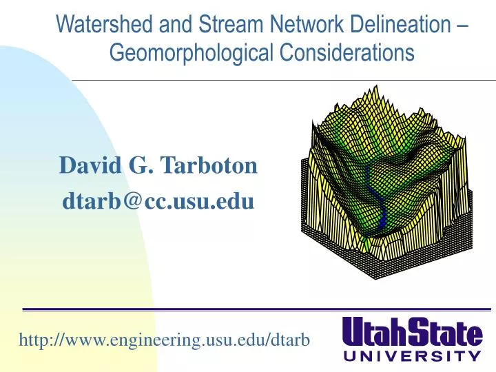
Watershed and Stream Network Delineation – Geomorphological Considerations. David G. Tarboton dtarb@cc.usu.edu. http://www.engineering.usu.edu/dtarb. Overview. Review of flow direction, accumulation and watershed delineation Topographic texture and drainage density

E N D
Watershed and Stream Network Delineation – Geomorphological Considerations David G. Tarboton dtarb@cc.usu.edu http://www.engineering.usu.edu/dtarb
Overview • Review of flow direction, accumulation and watershed delineation • Topographic texture and drainage density • Channel network geomorphology and Hortons Laws • Stream drop test to objectively oelect channel delineation threshold • Curvature and slope based methods to represent variable drainage density • The D approach • Specialized grid accumulation functions • TauDEM software
Elevation Surface — the ground surface elevation at each point Digital Elevation Model — A digital representation of an elevation surface. Examples include a (square) digital elevation grid, triangular irregular network, set of digital line graph contours or random points.
Digital Elevation Grid — a grid of cells (square or rectangular) in some coordinate system having land surface elevation as the value stored in each cell. Square Digital Elevation Grid — a common special case of the digital elevation grid
67 56 49 52 48 37 58 55 22 Direction of Steepest Descent 30 30 67 56 49 52 48 37 58 55 22 Slope:
32 64 128 16 1 8 4 2 Eight Direction Pour Point Model ESRI Direction encoding
4 3 2 5 1 6 7 8 Eight Direction Pour Point Model D8 Band/GRASS/TARDEM Direction encoding
Contributing Area Grid 1 1 1 1 1 1 1 1 1 1 1 4 3 3 1 4 3 1 1 3 1 1 1 1 1 12 1 2 1 12 1 1 1 2 16 1 1 2 1 16 2 1 3 6 25 3 6 1 2 25 TauDEM convention includes the area of the grid cell itself.
4 3 2 5 1 6 7 8 Direction encoding 1 2 3 1 1 7 6 5 2 1 7 6 5 3 6 7 7 Contributing area Programming the calculation of contributing area 2 2 3 6
1 1 1 1 1 1 4 3 3 1 1 2 1 1 12 1 1 1 2 16 2 1 3 6 25 Contributing Area > 10 Cell Threshold
100 grid cell constant support area threshold stream delineation
200 grid cell constant support area based stream delineation
AREA 2 3 AREA 1 12 How to decide on support area threshold ? Why is it important?
Hydrologic processes are different on hillslopes and in channels. It is important to recognize this and account for this in models. Drainage area can be concentrated or dispersed (specific catchment area) representing concentrated or dispersed flow.
Delineation of Channel Networks and Subwatersheds 500 cell theshold 1000 cell theshold
Examples of differently textured topography Badlands in Death Valley.from Easterbrook, 1993, p 140. Coos Bay, Oregon Coast Range. from W. E. Dietrich
Canyon Creek, Trinity Alps, Northern California. Photo D K Hagans
Gently Sloping Convex Landscape From W. E. Dietrich
Same scale, 20 m contour interval Driftwood, PA Sunland, CA Topographic Texture and Drainage Density
“landscape dissection into distinct valleys is limited by a threshold of channelization that sets a finite scale to the landscape.” (Montgomery and Dietrich, 1992, Science, vol. 255 p. 826.) Lets look at some geomorphology. • Drainage Density • Horton’s Laws • Slope – Area scaling • Stream Drops Suggestion:One contributing area threshold does not fit all watersheds.
Drainage Density • Dd = L/A • Hillslope length 1/2Dd B B Hillslope length = B A = 2B L Dd = L/A = 1/2B B= 1/2Dd L
Drainage Density for Different Support Area Thresholds EPA Reach Files 100 grid cell threshold 1000 grid cell threshold
Hortons Laws: Strahler system for stream ordering 1 3 1 2 1 2 1 1 1 1 1 2 2 1 1 1 1 1 1
Slope-Area scaling Data from Reynolds Creek 30 m DEM, 50 grid cell threshold, points, individual links, big dots, bins of size 100
Constant Stream Drops Law Broscoe, A. J., (1959), "Quantitative analysis of longitudinal stream profiles of small watersheds," Office of Naval Research, Project NR 389-042, Technical Report No. 18, Department of Geology, Columbia University, New York.
Nodes Links Single Stream Note that a “Strahler stream” comprises a sequence of links (reaches or segments) of the same order Stream DropElevation difference between ends of stream
Look for statistically significant break in constant stream drop property Break in slope versus contributing area relationship Physical basis in the form instability theory of Smith and Bretherton (1972), see Tarboton et al. 1992 Suggestion: Map channel networks from the DEM at the finest resolution consistent with observed channel network geomorphology ‘laws’.
T-Test for Difference in Mean Values 72 130 0 T-test checks whether difference in means is large (> 2) when compared to the spread of the data around the mean values
200 grid cell constant support area based stream delineation
Local Curvature Computation(Peuker and Douglas, 1975, Comput. Graphics Image Proc. 4:375) 43 48 48 51 51 56 41 47 47 54 54 58
Channel network delineation, other options 4 3 2 1 1 1 1 1 1 1 1 1 1 5 6 7 1 1 1 4 2 3 2 2 3 1 1 Grid Order 8 1 1 1 2 1 1 1 1 3 12 1 1 1 1 1 1 2 1 16 3 1 2 1 1 2 3 6 2 25 3 Contributing Area
? Topographic Slope Topographic Definition Drop/Distance Limitation imposed by 8 grid directions. Flow Direction Field — if the elevation surface is differentiable (except perhaps for countable discontinuities) the horizontal component of the surface normal defines a flow direction field.
The D Algorithm Tarboton, D. G., (1997), "A New Method for the Determination of Flow Directions and Contributing Areas in Grid Digital Elevation Models," Water Resources Research, 33(2): 309-319.) (http://www.engineering.usu.edu/cee/faculty/dtarb/dinf.pdf)