Download

1 / 19
290 likes | 877 Views
Discontinuous Galerkin Methods. Li, Yang FerienAkademie 2008. Contents. Methods of solving PDEs. Introduction of DG Methods. Working with 1-Dimension. Methods of solving PDEs. Finite Difference Method. PDEs. Finite Volume Method. Finite Element Method. Methods of solving PDEs.

E N D
Discontinuous Galerkin Methods Li, Yang FerienAkademie 2008
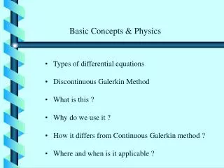
Contents Methods of solving PDEs Introduction of DG Methods Working with 1-Dimension
Methods of solving PDEs Finite Difference Method PDEs Finite Volume Method Finite Element Method
Methods of solving PDEs • E.g. 1D scalar conservation law with initial conditions and boundary conditions on the boundary unknown solution flux prescribed force How to get the approximate solution ? Is it satisfied the equation?
Methods of solving PDEs • Finite Difference Method a grid local grid size assume: Residual:
Methods of solving PDEs Element-based discretization to ensure geometry flexibility Finite Difference Method Simple to implement Ill-suited to deal with complex geometries
Divergence Theorem Reconstruction of Solution To find the p+1 unknown coefficients need information at least from p+1 cells Methods of solving PDEs • Finite Volume Method element staggered grid , solution is approximated on the element by a constant The actual numerical scheme will depend upon problem geometry and mesh construction. Difficult when high-order reconstruction.
Methods of solving PDEs • Finite Element Method assume the local solution: element locally defined basis function global representation of : where is the basis function. define a space of test functions, , and require the residual is orthogonal to all test functions:
Methods of solving PDEs • Finite Element Method Classical choice: the spaces spanned by the basis functions and test functions are the same. Since the residual has to vanish for all Easy to extend to high-order approximation by adding additional degrees of freedom to the element. The semi-discrete scheme becomes implicit and M must be inverted
Introduction of DG Methods • The Discontinuous Galerkin method is somewhere between a finite element and a finite volume method and has many good features of both, utilizing a space of basis and test functions that mimics the finite element method but satisfying the equation in a sense closer to the finite volume method. • It provides a practical framework for the development of high-order accurate methods using unstructured grids. The method is well suited for large-scale time-dependent computations in which high accuracy is required. • An important distinction between the DG method and the usual finite-element method is that in the DG method the resulting equations are local to the generating element. The solution within each element is not reconstructed by looking to neighboring elements. Its compact formulation can be applied near boundaries without special treatment, which greatly increases the robustness and accuracy of any boundary condition implementation.
Introduction of DG Methods • From FEM and FVM to DG-FEM maintain the definition of elements as in the FEM but new definition of vector of unknowns Assume the local solution in each element is: (likewise for the flux) Define The space of basis functions: The local residual is:
Introduction of DG Methods Require that the residual is orthogonal to all test functions : Similar to FVM, use Gauss’ theorem: introduce the numerical flux, , as the unique value to be used at the interface and obtained by coming information from both elements. applying Gauss’ theorem again: Weak Form Strong Form
Introduction of DG Methods • More general form Consider the nonlinear, scalar, conservation law: subject to appropriate initial conditions The boundary conditions are provided when the boundary is an inflow boundary: when when We still assume that the global solution can be well approximated by a space of piecewise polynomial functions, defined on the union of , and require the residual to be orthogonal to space of the test functions,
Introduction of DG Methods recover the locally defined weak formulation: and the strong form: Assume that all local test functions can be represented by using a local polynomial basis, , as and leads to equations as:
Working with 1-Dimension E.g. • Choose the basis functions: Jacobi polynomials • Integral: Gaussian quadrature • Time: 4th order explicit RK method • Simple algorithm steps: Generate simple mesh Construct the matrices Solve the equation system
Reference • Jan S Hesthaven, Tim Warburton: Nodal Discontinuous Galerkin Methods: Algorithms, Analysis, and Applications, Springer • Cockburn B, Shu CW: TVB Runge-Kutta local projection discontinuous Galerkin finite element method for conservation laws II: general framework, MATHEMATICS OF COMPUTATION, v52 (1989), pp.411-435. • http://lsec.cc.ac.cn/lcfd/DGM_mem.html • http://www.wikipedia.org/ • http://www.nudg.org/