Download
1 / 48
480 likes | 697 Views
High Resolution Aerospace Applications using the NASA Columbia Supercomputer. Dimitri J. Mavriplis University of Wyoming Michael J. Aftosmis NASA Ames Research Center Marsha Berger Courant Institute, NYU. Computational Aerospace Design and Analysis.

E N D
High Resolution Aerospace Applications using the NASA Columbia Supercomputer Dimitri J. Mavriplis University of Wyoming Michael J. Aftosmis NASA Ames Research Center Marsha Berger Courant Institute, NYU
Computational Aerospace Design and Analysis • Computational Fluid Dynamics (CFD) Successes • Preliminary design estimates for various conditions • Accurate prediction at cruise conditions (no flow separation)
Computational Aerospace Design and Analysis • Computational Fluid Dynamics (CFD) Successes • Preliminary design estimates for various conditions • Accurate prediction at cruise conditions (no flow separation) • CFD Shortcomings • Poor predictive ability at off-design conditions • Complex geometry, flow separation • High accuracy requirements: • Drag coefficient to 10-4 (i.e. wind tunnels) • Production runs with 109 grid points (vs 107 today) should become commonplace (NIA Congressional Report, 2005)
Computational Aerospace Design and Analysis • Computational Fluid Dynamics (CFD) Successes • Preliminary design estimates for various conditions • Accurate prediction at cruise conditions (no flow separation) • CFD Shortcomings • Poor predictive ability at off-design conditions • Complex geometry, flow separation • High accuracy requirements: • Drag coefficient to 10-4 (i.e. wind tunnels) • Production runs with 109 grid points (vs 107 today) should become commonplace (NIA Congressional Report, 2005) • Drive towards Simulation based Design • Design Optimization (20 – 100 Analyses) • Flight envelope simulation (103 – 106 Analyses) • Unsteady Simulations • Aeroelastics • Digital Flight (simulation of maneuvering vehicle)
MOTIVATION • CFD computational requirements in aerospace vehicle design are essentially insatiable for the foreseeable future • Addressable through hardware and software (algorithmic) advances • Recently installed NASA Columbia Supercomputer provides quantum leap in agency’s/stakeholders’ computing capability • Demonstrate advances in state-of-the-art using 2 production codes on Columbia • Cart3D (NASA Ames, NYU) • Lower Fidelity, rapid turnaround anaysis • NSU3D (ICASE/NASA Langley, U. Wyoming) • Higher Fidelity, analysis and design
Cart3D: Cartesian Mesh Inviscid Flow Simulation Package • Unprecedented level of automation • Inviscid analysis package • Surface modeling, mesh generation, data extraction • Insensitive to geometric complexity • Aimed at: • Aerodynamic database generation • Parametric studies • Preliminary design • Wide dissemination • NASA, DoD, DOE, Intel Agencies • US Aerospace industry, commercial and general aviation Parametric Analysis Flow solution Domain Decomposition Mesh Generation
Partition 0 Partition 1 Fine Coarse Each subdomain resides in processor local memory • Space-Filling-Curve based partitioner and mesh coarsener • Each subdomain has own local grid hierarchy • Good (not perfect) nesting – favor load balance at each level • Restrict use of OpenMP constructs - Use MPI-like architecture • Exchange via structure copy (OpenMP), send/receive (MPI) Cart3D Solver programming paradigm Explicit subdomain communication
Flight-Envelope Data-Base Generation (parametric analysis) • Configuration space • Vary geometric parameters • Control surface deflection • Shape optimization • Requires remeshing • Wind-Space Parameters • Vary wind vector • Mach, a:incidence, b:sideslip • No remeshing • Completely Automated • Hierarchical Job launching, scheduling • Data retrieval
Aerodynamic Database Generation Parametric Analysis
Flight-Envelope Data-Base Generation (parametric analysis) • Configuration space • Vary geometric parameters • Control surface deflection • Shape optimization • Requires remeshing • Wind-Space Parameters • Vary wind vector • Mach, a:incidence, b:sideslip • No remeshing • Completely Automated • Hierarchical Job launching, scheduling • Data retrieval
• Wind-Space: M∞ ={0.2-6.0}, α ={-5°–30°}, b ={0°–30°} • P has dimensions (38 x 25 x 5) • 2900 simulations • Liquid glide-back booster - Crank delta wing, canards, tail • Wind-space only Database Generation parametric Analysis: Wind-Space
• Wind-Space: M∞ ={0.2-6.0}, α ={-5°–30°}, b ={0°–30°} • P has dimensions (38 x 25 x 5) • 2900 simulations • Liquid glide-back booster - Crank delta wing, canards, tail • Wind-space only • Typically smaller resolution runs • 32-64 cpus each • Farmed out simultaneously (PBS) • 2900 simulations
• Wind-Space: M∞ ={0.2-6.0}, α ={-5°–30°}, b ={0°–30°} • P has dimensions (38 x 25 x 5) • 2900 simulations • Liquid glide-back booster - Crank delta wing, canards, tail • Wind-space only • Need for higher resolution simulations • - Selected data-base points • - General drive to higher accuracy • Good large cpu count scalability important
NSU3D: Unstructured Navier-Stokes Solver • High fidelity viscous analysis • Resolves thin boundary layer to wall • O(10-6) normal spacing • Stiff discrete equations to solve • Suite of turbulence models available • High accuracy objective: 0.01% Cd • 50-100 times cost of inviscid analysis (Cart3D) • Unstructured mixed element grids for complex geometries • VGRID: NASA Langley • Production use in commercial, general aviation industry • Extension to Design Optimization and Unsteady Simulations
Agglomeration Multigrid • Agglomeration Multigrid solvers for unstructured meshes • Coarse level meshes constructed by agglomerating fine grid cells/equations
Agglomeration Multigrid • Automated Graph-Based Coarsening Algorithm • Coarse Levels are Graphs • Coarse Level Operator by Galerkin Projection • Grid independent convergence rates (order of magnitude improvement)
Anisotropy Induced Stiffness • Convergence rates for RANS (viscous) problems much slower then inviscid flows • Mainly due to grid stretching • Thin boundary and wake regions • Mixed element (prism-tet) grids • Use directional solver to relieve stiffness • Line solver in anisotropic regions
Strong coupling Method of Solution • Line-implicit solver
Parallelization through Domain Decomposition • Intersected edges resolved by ghost vertices • Generates communication between original and ghost vertex • Handled using MPI and/or OpenMP (Hybrid implementation) • Local reordering within partition for cache-locality • Multigrid levels partitioned independently • Match levels using greedy algorithm • Optimize intra-grid communication vs inter-grid communication
Partitioning • (Block) Tridiagonal Lines solver inherently sequential • Contract graph along implicit lines • Weight edges and vertices • Partition contracted graph • Decontract graph • Guaranteed lines never broken • Possible small increase in imbalance/cut edges
Partitioning Example • 32-way partition of 30,562 point 2D grid • Unweighted partition: 2.6% edges cut, 2.7% lines cut • Weighted partition: 3.2% edges cut, 0% lines cut
Hybrid MPI-OMP (NSU3D) • MPI master gathers/scatters to OMP threads • OMP local thread-to-thread communication occurs during MPI Irecv wait time (attempt to overlap)
Simulation Strategy • NSU3D: Isolated high resolution analyses and design optimization • Cart3D: Rapid flight envelope data-base fill-in • Examine performance of each code individually on Columbia • Both codes use customized multigrid solvers • Domain-decomposition based parallelism • Extensive cache-locality reordering optimization • 1.3 to 1.6 Gflops on 1.6GHz Itanium2 cpu (pfmon utility) • NSU3D: Hybrid MPI/OpenMP • Cart3D: MPI or OpenMP (exclusively)
NASA Columbia Supercluster • 20 SGI Atix Nodes • 512 Itanium2 cpus each • 1 Tbyte memory each • 1.5Ghz / 1.6Ghz • Total 10,240 cpus • 3 Interconnects • SGI NUMAlink (shared memory in node) • Infiniband (across nodes) • 10Gig Ethernet (File I/O) • Subsystems: • 8 Nodes: Double density Altix 3700BX2 • 4 Nodes: NUMAlink4 interconnect between nodes • BX2 Nodes, 1.6GHz cpus
NASA Columbia Subsystems • 4 Node: Altix 3700 BX2 • 2048 cpus, 1.6GHz, 4 Tbytes RAM • NUMAlink4 between all cpus (6.4Gbytes/s) • MPI, SHMEM, MLP across all cpus • OpenMP (OMP) within a node • Infiniband using MPI across all cpus • Limited to 1524 mpi processes • 8 Node: Altix 3700BX2 • 4096 cpus, 1.6 GHz / 1.5 GHz, 8 Tbytes RAM • Infiniband using MPI required for cross-node communication • Hardware limitation: 2048 MPI connections • Requires hybrid MPI/OMP to access all cpus • 2 OMP threads running under each MPI process • Overall well balanced machine: • 1Gbyte/sec I/O on each node
Cart3D Solver Performance • Test problem: • Full Space Shuttle Launch Vehicle • Mach 2.6, • AoA = 2.09 deg • Mesh 25 M cells
Cart3D Solver Performance Pressure Contours • Test problem: • Full Space Shuttle Launch Vehicle • Mach 2.6, • AoA = 2.09 deg • Mesh 25 M cells
Cart3D Solver Performance Compare OpenMP and MPI • Pure OpenMP restricted to single 512 cpu node • Ran from 32-504 cpus (node c18) • Perfect speed-up assumed on 32 cpus • OpenMP show slight beak at 128 cpus due to change in global addressing scheme - MPI unaffected (no global addressing) • MPI achieves ~0.75 TFLOP/s on 496 cpus
Cart3D Solver Performance Single Mesh vs Multigrid • Used NUMAlink on c17-c20 • MPI only, from 32-2016 cpus • Reducing multigrid de-emphasizes communication • Single-grid scalability ~1900 on 2016 cpus • Coarsest mesh in 4 level multigrid has ~16 cells/partition • 4 Level multigrid shows parallel speedups of 1585 on 2016 cpus
Cart3D Solver Performance Compare NUMAlink & Infiniband • MPI only, from 32-2016 cpus, 4 Level multigrid • 32-496 cpus run on 1 node - (no interconnect) • 508-1000 cpus run on 2 nodes • 1000-2016 cpus on 4 nodes • IB lags due to decrease in delivered bandwidth • Delivered bandwidth drops again when going from 2 to 4 nodes • NUMAlink on 2016 cpus achieves over 2.4 TFLOP/s
NSU3D TEST CASE • Wing-Body Configuration • 72 million grid points • Transonic Flow • Mach=0.75, Incidence = 0 degrees, Reynolds number=3,000,000
NSU3D Scalability G F L O P S • 72M pt grid • Assume perfect speedup on 128 cpus • Good scalability up to 2008 using NUMAlink • Superlinear ! • Multigrid slowdown due to coarse grid communication • ~3TFlops on 2008 cpus
NSU3D Scalability • Best convergence with 6 level multigrid scheme • Importance of fastest overall solution strategy • 5 level Multigrid • 10 minutes wall clock time for steady-state solution on 72M pt grid
NUMAlink vs. Infiniband (IB) • IB required for > 2048 cpus • Hybrid MPI/OMP required due to MPI limitation under IB • Slight drop-off using IB • Additional penalty with increasing OMP Threads • (locally) sequential nature during mpi to mpi communication 128 cpu run split across 4 hosts
NUMAlink vs. Infiniband (IB) Single Grid (no multigrid) • 2 OMP required for IB on 2048 • Excellent scalability for single grid solver (non multigrid)
NUMAlink vs. Infiniband (IB) 6 level multigrid • 2 OMP required for IB on 2048 • Dramatic drop-off for 6 level multigrid
NUMAlink vs. Infiniband(IB) 5 level multigrid • 2 OMP required for IB on 2048 • Dramatic drop-off for 5 level multigrid
NUMAlink vs. Infiniband(IB) 4 level multigrid • 2 OMP required for IB on 2048 • Dramatic drop-off for 4 level multigrid
NUMAlink vs. Infiniband(IB) 3 level multigrid • 2 OMP required for IB on 2048 • Dramatic drop-off for 3 level multigrid
NUMAlink vs. Infiniband(IB) 2 level multigrid • 2 OMP required for IB on 2048 • Dramatic drop-off for 2 level multigrid
NUMAlink vs. Infiniband(IB) 2nd coarse grid level alone ( < 1M pts) • Similar slowdowns with NUMALINK and Infiniband
NUMAlink vs. Infiniband(IB) • Inconsistent NUMAlink/Infiniband performance • Multigrid IB drop-off not due to coarse grid level communication • Due to inter-grid communication • Not bandwidth related • More non-local communication pattern • Sensitive to system ENV variable settings • Addressable through: • More local fine to coarse partitioning • Multi-level communication strategy
Single Grid Performance up to 4016 cpus • 1 OMP possible for IB on 2008 (8 hosts) • 2 OMP required for IB on 4016 (8 hosts) • Good scalability up to 4016 • 5.2 Tflops at 4016 First real world application on Columbia using > 2048 cpus
Inhomogeneous CPU Set • 1.5GHz (6Mbyte L3) cpus vs 1.6GHz (9Mbyte L3) cpus • Responsible for part of slowdown
Concluding Remarks • NASA’s Columbia Supercomputer enabling advances in state-of-the-art for aerospace computing applications • ~100M grid point solutions (turbulent flow) in 15 minutes • Design Optimization overnight (20-100 analyses) • Rapid flight envelope data-base generation • Time dependent maneuvering solutions: • Digital Flight
Conclusions • Much higher resolution analyses possible • 72M pts on 4016 cpus only 18,000 points per cpu • 109 Grid points feasible on 2000+ cpus • Should become routine in future • Approximately 4 hour turnaround on Columbia • Other bottlenecks must be addressed • I/O Files: 35 Gbytes for 72M pts -- 400Gbytes for 109pts • Other sequential pre/post processing (i.e. grid generation) • Requires rethinking entire process • On demand parallel grid refinement and load balancing • Obviates large input files • Requires link to CAD database from parallel machine
Conclusions • Columbia Supercomputer Architecture validated on real world applications (2 production codes) • NUMAlink provides best performance but currently limited to 2048 cpus • Infiniband practical for very large applications • Requires hybrid MPI/OMP communication • Issues remain concerning communication patterns • Bandwidth adequate for current and larger applications • Large applications on 8,000 to 10,240 cpus using IB and OMP 4 should be feasible and achieve ~12Tflops • Special thanks to : Bob Ciotti (NASA), Bron Nelson (SGI)