Download
1 / 51
510 likes | 648 Views
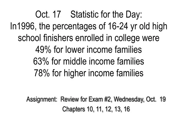
Oct. 17 Statistic for the Day: In1996, the percentages of 16-24 yr old high school finishers enrolled in college were 49% for lower income families 63% for middle income families 78% for higher income families. Assignment: Review for Exam #2, Wednesday, Oct. 19 Chapters 10, 11, 12, 13, 16.

E N D
Oct. 17 Statistic for the Day:In1996, the percentages of 16-24 yr old high school finishers enrolled in college were49% for lower income families63% for middle income families78% for higher income families Assignment: Review for Exam #2, Wednesday, Oct. 19 Chapters 10, 11, 12, 13, 16
Arby’s sandwiches weight calories 1 Big Montana 309 g 590 2 Giant Roast Beef 224 450 3 Regular Roast Beef 154 320 4 Beef ‘n Cheddar 195 440 5 Super Roast Beef 230 440 6 Junior Roast Beef 125 270 7 Chicken Breast Fillet 233 500 8 Chicken Bacon ‘n Swiss 209 550 9 Roast Chicken Club 228 470 10 Market Fresh Turkey Ranch Bacon 379 830 11 Market Fresh Ultimate BLT 293 780 12 Market Fresh Roast Beef Swiss 357 780 13 Market Fresh Roast Ham Swiss 357 700 14 Market Fresh Roast Turkey Swiss 357 720 15 Market Fresh Chicken Salad 322 770
This type of plot, with two measurements per subject, is called a scatterplot (see p. 166).
The correlation measures the strength of the linear relationship between weight and calories. More on this in the next class.
The best-fitting line through the data is called the regression line. How should we describe this line?
The intercept is 18 in this case and the slope is 2.1. In this class, you don’t need to know how to calculate the slope and intercept (but see p. 195 if you like formulas).
intercept slope calories = 18 + (2.1)(weight in grams) ------------------------------------------------- For example, if you have a 200g sandwich, on the average you expect to get about: 18 + (2.1)(200) = 18 + 420 = 438 calories -------------------------------------------------- For a 350g sandwich: 18 + (2.1)(350) = 18 + 735 = 753 calories
intercept slope calories = 18 + (2.1)(weight in grams) For every extra gram of weight, you expect an increase of 2.1 calories in your Arby’s sandwich. Interpretation of slope: Expected increase in response for every unit increase (increase of one) in explanatory.
Facts about Correlation: • +1 means perfect increasing linear relationship • -1 means perfect decreasing linear relationship • 0 means no linear relationship • + means increasing together • - means one increases and the other decreases
Strength vs. statistical significance • Even a weak relationship can be statistically significant (if it is based on a large sample) • Even a strong relationship can be statistically insignificant (if it is based on a small sample)
Regression potential pitfalls: Sometimes we see strong relationship in absurd examples; two seemingly unrelated variables have a high correlation. This signals the presence of a third variable that is highly correlated with the other two (confounding). Remember that correlation does not imply causation. Also: If you use a regression for prediction, do not extrapolate too far beyond the range of the observed data.
Outliers Outliers are data that are not compatible with the bulk of the data. They show up in graphical displays as detached or stray points. Sometimes they indicate errors in data input. Some experts estimate that roughly 5% of all data entered is in error. Sometimes they are the most important data points.
Put Options (NYTimes, September 26, 2001) Put options on stocks give buyers the right to sell stock at a specified price during a certain time. They rise in value if the underlying stock falls below the strike price. The value of puts on airline stocks soared on Sept. 17 when U.S. stock and options markets reopened after a four-day closure, as airline stocks slid as much as 40 percent. American Airlines was at $32 prior to attack. Suppose a terrorist buys a put option (at say $5 per share) to have the right to sell at $25. The price after the attack was at $16. That put option is now more valuable.
R wins machine (D minus R negative for machine) D wins absentee (D minus R positive for absentee) From story on p. 442
Outliers affect regression lines and correlation (these data aren’t real): Red line: Without A, with B Black line: With A and B Green line: Without A or B
Two categorical variables: Explanatory variable: SexResponse variable: Body Pierced or Not Survey question: Have you pierced any other part of your body? (Except for ears) Research Question: Is there a significant difference between women and men at PSU in terms of body pierces?
Data: Response: Body Pierced? Explanatory: Sex From STAT 100, fall 2005 (missing responses omitted)
Percentages Response: body pierced? no yes All female 62.32% 37.68% 100.00% male 93.90% 6.10% 100.00% All 74.09% 25.91% 100.00% 62.32% = 86 / 138 93.90% = 77 / 82 Research question: Is there a significant difference Between women and men? (i.e., between 66.67% and 91.35%)
The Debate: The research advocate claims that there is a significant difference. The skeptic claims there is no real difference. The data differences simply happen by chance, since we’ve selected a random sample.
The strategy for determining statistical significance: • First, figure out what you expect to see if there is no difference between females and males • Second, figure out how far the data is from what is expected. • Third, decide if the distance in the second step is large. • Fourth, if large then claim there is a statistically significant difference.
Exercise:Follow the 4 steps and answer theResearch Question: Is there a statistically significant difference between males and females in terms of the percent who have used marijuana? Data from STAT 100 fall 2005 Rows: Sex Columns: Marijuana No Yes All Female 56 76 132 Male 31 46 77 All 87 122 209
Step 1: Find expected counts if the skeptic is correct This step is based on the marginal totals: (Repeat for B, C, D) A =
Step 1 cont’d Repeat the process for B (and then C and D): Or you can simply subtract: 132 – 54.95 = 77.05 B =
Step 1 cont’d Green: Observed counts Red: Expected counts if skeptic is correct. Marijuana? No Yes All Female 56 76 132 54.95 77.05 132.00 Male 31 46 77 32.05 44.95 77.00 Total 87 122 209
Step 2: How far are the data (observed counts) from what is expected? Green: Observed counts Red: Expected counts if skeptic is correct. Chi-Sq = 0.020 + 0.014 + 0.034 + 0.025 = 0.093
Step 3: Is the distance in step 2 large? Something is large when it is in the outer 5% tail of the appropriate distribution. Chi-squared distribution with 1 degree of freedom: If chi-squared statistic is larger than 3.84, it is declared large and the research advocate wins. Our chi-squared value: 0.093 (from Step 2)
Step 4: If distance is large, claim statistically significant difference. Rows: Sex Columns: marijuana No Yes All Female 56 76 132 42.4% 57.6% 100.0% Male 31 46 77 40.3% 59.7% 100.0% Hence, the difference: 57.6% of women versus 59.7% of men is not statistically significant in this case. (Sample size has been automatically considered!)
How many degrees of freedom here? Degrees of freedom (df) always equal (Number of rows – 1) × (Number of columns – 1)
Health studies and risk Research question: Do strong electromagnetic fields cause cancer? 50 dogs randomly split into two groups: no field, yes field The response is whether they get lymphoma. Rows: mag field Columns: cancer no yes All no 20 5 25 yes 10 15 25 All 30 20 50
Terminology and jargon: In the mag field group, 15/25 of the dogs got cancer. Therefore, the following are all equivalent: • 60% of the dogs in this group got cancer. • The proportion of dogs in this group that got cancer is 0.6. • The probability that a dog in this group got cancer is 0.6. • The risk of cancer in this group is 0.6 And one more: The odds of cancer in this group are 3/2.
More terminology and jargon: • Identify the ‘bad’ response category: In this example, cancer • Treatment risk: 15 / 25 or .60 or 60% • Baseline risk: 5 / 25 or .20 or 20% • Relative risk: Treatment risk over Baseline risk = .60 / .20=3 That is, the treatment risk is three times as large as the baseline risk. • Increased risk: By how much does the risk increase for treatment as compared to control? (.60 - .20) / .20 = 2 or 200% That is, the risk is 200% higher in the treatment group. • Odds ratio: Ratio of treatment odds to baseline odds. (15/10) / (5/20) turns out to be 6. That is, the treatment odds are six times as large as the baseline odds.
Final note: When the chi-squared test is statistically significant then it makes sense to compute the various risk statements. If there is no statistical significance then the skeptic wins. There is no evidence in the data for differences in risk for the categories of the explanatory variable.
Recall marijuana example Marijuana? No Yes All Female 56 76 132 54.95 77.05 132.00 Male 31 46 77 32.05 44.95 77.00 Total 87 122 209 Chi-Sq = 0.020 + 0.014 + 0.034 + 0.025 = 0.093 SO THE SKEPTIC WINS. But what if we observed a much larger sample? Say, 100 times larger?
Marijuana example, larger sample: Marijuana? No Yes All Female 5600 7600 13200 5495 7705 13200 Male 3100 4600 7700 3205 4495 7700 Total 8700 12200 20900 Chi-Sq = 2.0 + 1.4 + 3.4 + 2.5 = 9.3 NOW THE RESEARCH ADVOCATE WINS.
Practical significance In the marijuana example, 58% of women and 60% of men reported that they had tried marijuana. This size of difference, even if it is really in the population, is probably uninteresting. Yet we have seen that a large sample size can make it statistically significant. Hence, in the interpretation of statistical significance, we should also address the issue of practical significance. In other words, we should answer the skeptic’s second question: WHO CARES?
Simpson’s paradox (for quantitative variables) Example 11.4, pp. 204-205 Correlation= -.312
Simpson’s paradox (for quantitative variables) Example 11.4, pp. 204-205 Correlation= -.312 H Correlation= .348 S Correlation= .637
Simpson’s paradox for categorical variables, as seen in video Overall admitted to City U. Business (hard) Law (easy) Women better in each, but more men apply to easier law school!
Rules: For combining probabilities 0 < Probability < 1 • If there are only two possible outcomes, then their probabilities must sum to 1. • If two events cannot happen at the same time, they are called mutually exclusive. The probability of at least one happening (one or the other) is the sum of their probabilities. [Rule 1 is a special case of this.] • If two events do not influence each other, they are called independent. The probability that they happen at the same time is the product of their probabilities. • If the occurrence of one event forces the occurrence of another event, then the probability of the second event is always at least as large as the probability of the first event.
Rule 1: If there are only two possible outcomes, then their probabilities must sum to 1. According to Example 3, page 302: P(lost luggage) = 1/176 = .0057 Thus, P(luggage not lost) = 1 – 1/176 = 175/176 = .9943 The point of rule 1 is that P(lost) + P(not lost) = 1 so if we know P(lost), then we can find P(not lost). Sounds simple, right? It can be surprisingly powerful.
Rule 2: If two events cannot happen at the same time, they are called mutually exclusive. In this case, the probability of at least one happening is the sum of their probabilities. [Rule 1 is a special case of this.] Example 5, page 303: Suppose P(A in stat) = .50 and P(B in stat) = .30. Then P( A or B in stat) = .50 + .30 = .80 Note that the events ‘A in stat’ and ‘B in stat’ are mutually exclusive. Do you see why?
Rule 3: If two events do not influence each other, they are called independent. In this case, the probability that they happen at the same time is the product of their probabilities. Example 8, page 303: Suppose you believe that P(A in stat) = .5 and P(A in history) = .6. Further, you believe that the two events are independent, so that they do not influence each other. Then P(A in stat and A in history) = (.5)×(.6) = .3 Is this a reasonable assumption?
Rule 4: If the occurrence of one event forces the occurrence of another event, then the probability of the second event is always at least as large as the probability of the first event. If event A forces event B to occur, then P(A) < P(B) Special case: P(E and F) < P(E) P(E and F) < P(F) (because ‘E and F’ forces E to occur).
Two laws (only one of them valid): • Law of large numbers: Over the long haul, we expect about 50% heads (this is true). • “Law of small numbers”: If we’ve seen a lot of tails in a row, we’re more likely to see heads on the next flip (this is completely bogus). Remember: The law of large numbers OVERWHELMS; it does not COMPENSATE.
The game of Odd Man Consider the “odd man” game. Three people at lunch toss a coin. The odd man has to pay the bill. You are the odd man if you get a head and the other two have tails or if you get a tail and the other two have heads. Notice that there will not always be an odd man – this occurs if flips come up HHH or TTT. P(no odd man) = P(HHH or TTT) = P(HHH) + P(TTT) since HHH, TTT are mutually exclusive = (1/2)3 + (1/2)3 since H,H,H are independent (as are T,T,T) =1/8 + 1/8 = .25 Thus, P(there is an odd man) = 1 – P(no odd man) = 1 - .25 = .75
Play until there is an odd man. What is the probability this will take exactly three tries? P(odd man occurs on the third try) = P(miss, miss, hit) in that order! That’s the only way. (See why?) = P(miss) P(miss) P(hit) since each try is independent of the others. = [P(miss)]2 P(hit) = [.25]2 .75 = .047 This is the final answer: The probability that the odd man occurs exactly on the third try (after two unsuccessful tries).
Expectation What if you bet $10 on a game of craps? What is your expected profit? (Probability of winning: 244/495, or 49.3%) You win $10 with probability .493 You lose $10 with probability .507 Expected profit: .493($10) + .507(-$10) = - $0.14
Casino winnings, 10,000 games per day Expectation = $1400
Casino winnings, 100,000 games a day Expectation = $14,000 Note: Now all values are positive