Download
1 / 11
110 likes | 251 Views
A Prescription for High-Redshift star formation. Alexander (Sasha) Muratov University of Michigan Advisor: Oleg Gnedin. Star Formation History of The Universe. Madau et al. 1996. State of Simulations.

E N D
A Prescription for High-Redshift star formation Alexander (Sasha) Muratov University of MichiganAdvisor: Oleg Gnedin
Star Formation History of The Universe Madau et al. 1996
State of Simulations Collisionless dark matter simulations can be run with great resolution down to zero redshift, but what are the stars and gas doing? Kravtsov et al. (2004)
Prescriptive Model: Advantages All quantities available at all times Made to be consistent with observations and simulations Can provide insight into global processes on different scales: Star Formation. Makes testable predictions. Disadvantages: makes testable predictions – need to match many data sets. Sometimes difficult to constrain.
Observed fits M*-Mh relation (Woo et al. 2008)logVc = -0.5 + .27logM* , M* ~ Vc3.8Vc = Vmax * 2½Mh ~ Vmax3.3 M*-Mgas relation (McGaugh 2005) Mass metallicity relation: Woo et al. (2008) Ms(z=0) = 109.6 MꙨ
Observed fits 2 – time evolution Dave & Oppenheimer (2007).3 dex lower over 10 Gyr Conroy & Wechsler (2008)Well fit by M* ~ (1+z)-2
Equations again Mass MW = 5.5 * 10^10 Solar (M*) MW = 1 * 10^10 Solar (Mgas) • Metallicity:extra constraints:
Anchored by GC's DM halos from Kravtsov et al. (2004) Hydro constraints from Kravtsov & Gnedin (2005) Bimodal metallicity distribution! (Muratov & Gnedin, in prep) KS Probablity: 51%
prediction for stellar fraction in dwarf galaxies M* = -1.85 + 1.03*Mh RMS: 0.212 Red Line : Andrey Kravtsov's relation (2009) Different techniques used: instead of matching brightest to most massive, we apply direct relations. Which is right?
Summary We present a prescriptive model for baryonic mass and metallicity as a function of time and halo mass. Applying this prescription to DM simulations, we have studied GC formation. We also obtain a fit for MW Dwarfs. Produces a different result from Kravtsov 2009, Busha 2009.