Download
1 / 1
10 likes | 149 Views
Three Particle Correlations as a Probe of Eccentricity Fluctuations Jim Thomas 1 and Paul Sorensen 2 for the STAR Collaboration 1 Lawrence Berkeley National Laboratory, 2 Brookhaven National Laboratory. Initial Density Fluctuations. Participant Eccentricity.

E N D
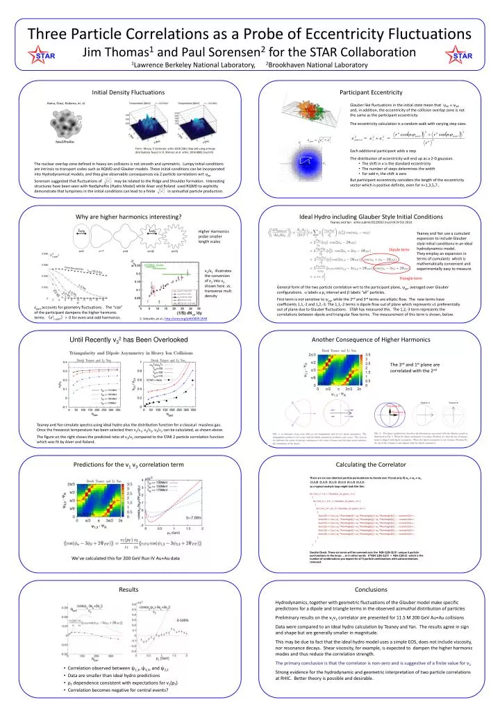
Three Particle Correlations as a Probe of Eccentricity Fluctuations Jim Thomas1 and Paul Sorensen2 for the STAR Collaboration 1Lawrence Berkeley National Laboratory, 2Brookhaven National Laboratory Initial Density Fluctuations Participant Eccentricity • Glauber like fluctuations in the initial state mean that PP RP and, in addition, the eccentricity of the collision overlap zone is not the same as the participant eccentricity • The eccentricity calculation is a random walk with varying step sizes. • Each additional participant adds a step • The distribution of eccentricity will end up as a 2-D gaussian. • The shift in x is the standard eccentricity • The number of steps determines the width • For odd n, the shift is zero • But participant eccentricity considers the length of the eccentricity vector which is positive definite, even for n=1,3,5,7… Hama, Grasi, Kodama, et. al. NexSPheRio From: Mocsy, P. Sorensen: arXiv:1008.3381 [hep-ph] using entropy distributions found in: K. Werner, et al. arXiv: 1004.0805 [nucl-th] The nuclear overlap zone defined in heavy ion collisions is not smooth and symmetric. Lumpy initial conditions are intrinsic to transport codes such as RQMD and Glauber models. These initial conditions can be incorporated into Hydrodynamical models; and they give observable consequences via 2 particle correlations wrtpp Sorensen suggested that fluctuations of may be related to the Ridge and Shoulder formation. Interesting structures have been seen with NexSpheRio (Hydro Model) while Alver and Roland used RQMD to explicitly demonstrate that lumpiness in the initial conditions can lead to a finite in azimuthal particle production. Why are higher harmonics interesting? Ideal Hydro including Glauber Style Initial Conditions Teaney and Yan arXiv:submit/0123932 [nucl-th] 9 Oct 2010 Higher Harmonics probe smaller length scales Teaney and Yan use a cumulant expansion to include Glauber style initial conditions in an ideal hydrodynamics model. They employ an expansion in terms of cumulants which is mathematically convenient and experimentally easy to measure. Dipole term Point like particles v2/ε2illustrates the conversion of ε2 into v2 , shown here .vs. transverse mult. density Triangle term • General form of the two particle correlation wrt to the participant plane, pp, averaged over Glauber configurations. labels a pt interval and labels “all” particles. • First term is not sensitive to pp, while the 2nd and 3rd terms are elliptic flow. The new terms have coefficients 1,1,-2 and 1,2,-3.The 1,1,-2 terms is dipole flow out of plane which represents v1 preferentially out of plane due to Glauber fluctuations. STAR has measured this. The 1,2,-3 term represents the correlations between dipole and triangular flow terms. The measurement of this term is shown, below. εpart accounts for geometry fluctuations . The “size” of the participant dampens the higher harmonic terms. 〈ε2n,part〉> 0 for even and odd harmonics. S. Voloshin, et al., http://arxiv.org/pdf/0809.2949 Until Recently v32has Been Overlooked Another Consequence of Higher Harmonics The 3rd and 1st plane are correlated with the 2nd Teaney and Yan simulate spectra using ideal hydro plus the distribution function for a classical massless gas. Once the freezeout temperature has been selected then v1/1, v2/2, v3/3 can be calculated, as shown above. The figure on the right shows the predicted ratio of v3/v2 compared to the STAR 2 particle correlation function which was fit by Alver and Roland. Predictions for the v1 v3 correlation term Calculating the Correlator There are six non-identical particle permutations to iterate over if (and only if) w1 w2 w3 (1,2,3) (1,3,2) (2,1,3) (2,3,1) (3,1,2) (3,2,1) so a typical analysis loop might look like this: for ( Int_ti = 0 ; i < Number_of_pions ; i++ ) { for ( Int_t j = i+1 ; j < Number_of_pions ; j++ ) { for ( Int_t k = j+1 ; k < Number_of_pions ; k++ ) { Sum123 += Cos ( w1 *PionAngle[i] + w2 *PionAngle[j] + w3 *PionAngle[k] ) ; counter123++ ; Sum123 += Cos ( w1 *PionAngle[i] + w3 *PionAngle[j] + w2 *PionAngle[k] ) ; counter123++ ; Sum123 += Cos ( w2 *PionAngle[i] + w1 *PionAngle[j] + w3 *PionAngle[k] ) ; counter123++ ; Sum123 += Cos ( w2 *PionAngle[i] + w3 *PionAngle[j] + w1 *PionAngle[k] ) ; counter123++ ; Sum123 += Cos ( w3 *PionAngle[i] + w1 *PionAngle[j] + w2 *PionAngle[k] ) ; counter123++ ; Sum123 += Cos ( w3 *PionAngle[i] + w2 *PionAngle[j] + w1 *PionAngle[k] ) ; counter123++ ; } } } Double Check: These six terms will be summed over the N(N-1)(N-2)/3! unique 3 particle permutations in the loops … or in other words 6*N(N-1)(N-2)/3! = N(N-1)(N-2) which is the number of combinations you expect for all 3 particle combinations with autocorrelations removed. We’ve calculated this for 200 GeV Run IV Au+Au data Results Conclusions Hydrodynamics, together with geometric fluctuations of the Glauber model make specific predictions for a dipole and triangle terms in the observed azimuthal distribution of particles Preliminary results on the v1v3correlatorare presented for 11.5 M 200 GeVAu+Au collisions Data were compared to an ideal hydro calculation by Teaney and Yan. The results agree in sign and shape but are generally smaller in magnitude. This may be due to fact that the ideal hydro model uses a simple EOS, does not include viscosity, nor resonance decays. Shear viscosity, for example, is expected to dampen the higher harmonic modes and thus reduce the correlation strength. The primary conclusion is that the correlatoris non-zero and is suggestive of a finite value for v3 Strong evidence for the hydrodynamic and geometric interpretation of two particle correlations at RHIC. Better theory is possible and desirable. 0-100% • Correlation observed between ψ1,3, ψ3,3, and ψ2,2 • Data are smaller than ideal hydro predictions • pTdependence consistent with expectations for v1(pT) • Correlation becomes negative for central events?