Download
1 / 15
150 likes | 302 Views
Geometric (Classical) MultiGrid. Grid:. x=0. x=1. x 0. x 1. x 2. x i. x N-1. x N. local averaging. Let. Linear scalar elliptic PDE (Brandt ~1971). 1 dimension Poisson equation Discretize the continuum. Linear scalar elliptic PDE. 1 dimension Laplace equation

E N D
Grid: x=0 x=1 x0 x1 x2 xi xN-1 xN local averaging Let Linear scalar elliptic PDE (Brandt ~1971) • 1 dimension Poisson equation • Discretize the continuum
Linear scalar elliptic PDE • 1 dimension Laplace equation • Second order finite differenceapproximation => Solve a linear system of equations Not directly, but iteratively => Use Gauss Seidel pointwise relaxation
Influence of (pointwise) Gauss-Seidel relaxation on the error Poisson equation, uniform grid Error of initial guess Error after 5 relaxation Error after 10 relaxations Error after 15 relaxations
The basic observations of ML • Just a few relaxation sweeps are needed to converge the highly oscillatory components of the error => the error is smooth • Can be well expressed by less variables • Use a coarser level (by choosing every other line) for the residual equation • Smooth component on a finer level becomes more oscillatory on a coarser level => solve recursively • The solution is interpolated and added
~ ~ = + h h u u new old ~ ~ 2 h 2 h v v TWO GRID CYCLE Fine grid equation: 1. Relaxation Approximate solution: Smooth error: Residual equation: residual: 2. Coarse grid equation: Approximate solution: 3. Coarse grid correction: 4. Relaxation
~ ~ 2 2 h h v v MULTI-GRID CYCLE TWO GRID CYCLE Fine grid equation: 1 1. Relaxation Approximate solution: Smooth error: Residual equation: 2 residual: 2. Coarse grid equation: 3 4 Approximate solution: by recursion ~ ~ 5 = + 3. Coarse grid correction: h h u u new old 6 4. Relaxation Correction Scheme
h 2h . . . h0/4 h0/2 h0 * interpolation (order m) of corrections V-cycle: V(n1,n2) residual transfer enough sweeps or direct solver relaxation sweeps *
Coarsening Interpolate and relax G1 G1 Apply grids in all scales: 2x2, 4x4, … , n1/2xn1/2 G2 G2 Solve the large systems of equations by multigrid! G3 G3 Gl Gl Hierarchy of graphs
Linear (2nd order) interpolation in 1D F(x) x1 x x2
Bilinear interpolation (Ult,Vlt) (Urt,Vrt) (x1,y2) (x2,y2) i (x0,y0) S(i) (x1,y1) (x2,y1) (Ulb,Vlb) (Urb,Vrb) C(S(i))={rb,rt,lb,lt}
(Ult,Vlt) (Urt,Vrt) (x1,y2) (x2,y2) i (Ul,Vl) (Ur,Vr) (x0,y0) S(i) (x1,y1) (x2,y1) (Ulb,Vlb) (Urb,Vrb)
The fine and coarse Lagrangians For each square k add an equi-density constraint eqd(k) = current area + fluxes of in/out areas – allowed area = 0 is the bilinear interpolation from grid 2h to grid h At the end of the V-cycle interpolate back to (x,y)


![[PDF] Free Download The Classical Music Book By DK](https://cdn4.slideserve.com/8171133/slide1-dt.jpg)