Download
1 / 68
680 likes | 801 Views
Multifactorial Population Attributable Fractions: Approaches, Examples, and Issues to Consider. Deborah Rosenberg, PhD and Kristin Rankin, PhD Epidemiology and Biostatistics School of Public Health University of Illinois at Chicago.

E N D
Multifactorial Population Attributable Fractions: Approaches, Examples, and Issues to Consider Deborah Rosenberg, PhD and Kristin Rankin, PhD Epidemiology and Biostatistics School of Public Health University of Illinois at Chicago
Multifactorial Population Attributable Fractions: Approaches, Examples, and Issues to ConsiderWednesday, May 30th, 3:15-5:00pm Deborah Rosenberg, PhD Kristin Rankin, PhD Research Associate Professor Research Assistant Professor Division of Epidemiology and Biostatistics University of IL School of Public Health Training Course in MCH Epidemiology
Background • In any multivariable analysis, the goal is to generate unconfounded / independent estimates of effect for each of many factors, taking into account the relationships among and intersection of those factors. • Different analytic approaches are required to obtainthese mutually exclusive estimates according to whether ratio measures of association or population attributable fractions (PAFs) are of interest.
Background In contrast to relative risks or odds ratios the PAF is a function of both the magnitude of association and the prevalence of risk in the population The crude PAF (Levin, 1953): Extension to a multivariable PAF or Rothman Bruzzi
Background • When estimating relative risks or odds ratios, independence can be achieved through use of usual adjustment procedures to control for confounding: “Does a risk factor confer excess risk of disease for an individualafter holding all other factors constant?” • When estimating PAFs, usual adjustment does not result in mutually exclusive PAFs, nor does it address the dynamics of how the prevalence of risk factors might change in the population over time “How much will eliminating a risk factor reduce the prevalence of disease in the population given that disease may still occur in the presence of other risk factors that have not yet been eliminated?”
Background • After adjustment, both ratio measures and PAFs may be overestimates because of residual confounding. • For PAFs, overestimation is of greater concern because simple adjustment assumes that only the factor of interest will be eliminated—its prevalence will be reduced to 0—while the prevalence of other factors remain constant. • Concern about the precision of PAF estimates is also critical since these measures directly speak to the potential impact of public health action
Background Methods that go beyond the usual adjustment approach have been developed to handle the problem of obtaining mutually exclusive and mutually adjusted PAFs: • Modifiable risk factors are considered together as belonging to what might be called a “risk system” • Expected disease reduction due to elimination of any one risk factor is quantified by acknowledging every possible sequence for eliminating all factors in the “risk system” over time. • the maximum expected disease reduction due to elimination of all risk factors in the “risk system” can also be appropriately quantified
Organizing Factors into a Risk System: A Framework for Computing PAFs • “Adjusted” PAF: The PAF for eliminating a risk factor from a risk system after controlling for other factors (Miettenin, 1974) • Summary PAF: The PAF for the maximum expected disease reduction when all factors in a risk system are simultaneously eliminated (Bruzzi, 1985) • Component PAF: The separate PAF for every possible combination of exposure levels in the risk system (the set of joint and separate effects of risk factors) 7
Organizing Factors into a Risk System: A Framework for Computing PAFs • Sequential PAF: The PAF for eliminating a risk factor in a particular order from a risk system; sets of sequential PAFs comprise all possible removal sequences • Average PAF:The PAF summarizing all possible sequences for eliminating a single modifiable risk factor (Eide and Gefeller, 1995)
Organizing Factors into a Risk System: A Framework for Computing PAFs The Average PAF • The AvgPAF for a risk factor is both mutually exclusive and mutually adjusted • The sum of AvgPAFs for all modifiable risk factors in a system equals the summary PAF (sumPAF) for the risk system as a whole—the % of disease reduction expected if all of the factors are simultaneously and completely eliminated from the population
Example: Simultaneously Considering 3 Risk Factors for a Health Outcome Let 3 factors be called M1, M2, and M3 The SummaryPAF for this “risk system” can be partitioned into seven component PAFs: M1 and M2 and M3 What is the proportion M1 and M2 of disease attributable M1 and M3 to each combination M2 and M3 of risk factors? M1 alone M2 alone M3 alone
Summary PAF Partitioned into 7 Component PAFs 3 Risk Factors for an Outcome Summary PAF = 0.34 Component PAFs still fail to provide a single estimate of the impact of each factor
Example: Simultaneously Considering 3 Risk Factors for a Health Outcome The SummaryPAF for this “risk system” can be partitioned six different ways into threesequential PAFs Computation of sequential PAFs involves a series of subtractions of adjusted and/or summary PAFs based on repeatedly redefining the risk system and its corresponding Summary PAF in terms of particular combinations of risk factors
Example: Simultaneously Considering 3 Risk Factors for a Health Outcome Six Sequences for Three Risk Factors Sequence #1: Eliminate M1, then M2, then M3 Sequence #2: Eliminate M1, then M3, then M2 Sequence #3: Eliminate M2, then M1, then M3 Sequence #4: Eliminate M2, then M3, then M1 Sequence #5: Eliminate M3, then M1, then M2 Sequence #6: Eliminate M3, then M2, then M1 For each factor, there are two 1st sequential PAFs, two 2nd sequential PAFs, and two 3rd Sequential PAFs.
Example: Simultaneously Considering 3 Risk Factors for a Health Outcome EXAMPLE (Sequence #1):Eliminate M1, then M2, then M3 1st SeqPAF* (M1) = PAF(M1) adjusting for M2 & M3 and other covariates** 2nd SeqPAF (M2) = SumPAF(M1 & M2) adjusting for M3 and other covariates – PAF(M1) adjusting for M2 & M3 and other covariates 3rd SeqPAF (M3) = SumPAF (M1 & M2 & M3) – SumPAF(M1 & M2) adjusting for M3 and other covariates *“adjusted” PAF **covariates are unmodifiable factors
Example: Simultaneously Considering 3 Risk Factors for a Health Outcome EXAMPLE (Sequence #5):Eliminate M3, then M1, then M2 1st SeqPAF* (M3) = PAF(M3) adjusting for M1 & M2 and other covariates** 2nd SeqPAF (M1) = SumPAF(M3 & M1) adjusting for M2 and other covariates – PAF(M3) adjusting for M1 & M2 and other covariates 3rd SeqPAF (M2) = SumPAF(M1 & M2 & M3) – (SumPAF(M3 & M1) adjusting for M2 and other covariates *“adjusted” PAF **covariates are unmodifiable factors
Summary PAF Partitioned into Sequential PAFs for Sequences #1 and #5 3 Risk Factors for an Outcome: Summary PAF = 0.34 Sequential PAFs still fail to provide a single estimate of the impact of each factor
Example: Simultaneously Considering 3 Risk Factors for a Health Outcome In general: the number of possible sequences is a function of the number of factors in the risk system and becomes large quickly as the number of variables increases.
Example: Simultaneously Considering 3 Risk Factors for a Health Outcome The SummaryPAF for this “risk system” can be partitioned into three average PAFs--onefor each of the 3 factors The sequences are broken apart, rearranging the sequential PAFs so that the six 1st, 2nd, and 3rd sequential PAFs for M1 are grouped together as are those for M2 and M3 The AveragePAF for each factor is then calculated as the simple arithmetic average across the 6 sequential PAFs for each factor
Example: Simultaneously Considering 3 Risk Factors for a Health Outcome For example, the Average PAF for M1 is the sum of the following 6 Sequential PAFs divided by 6: The two 1st SeqPAFs for M1—Seq #1 & Seq #2 = PAF(M1), adjusting** for M2 & M3 (multiplied by 2) The two 2nd SeqPAFs for M1—Seq #3 & Seq #5 = (SumPAF(M2 & M1), adj. for M3) – PAF(M2) adj. for M1 & M3 = (SumPAF(M3 & M1), adj. for M2) – PAF(M3) adj. for M1 & M2 The two 3rd SeqPAFs for M1—Seq #4 & Seq #6 = (SumPAF(M1 & M2 & M3) – SumPAF(M2 & M3), adj. for M1 **Adjustment also includes covariates
Summary PAF Partitioned into Average PAFs for Three Risk Factors The avgPAF for a factor is the simple average of all of that factor’s seqPAFs With 3 factors, the avgPAF 3 Risk Factors for an Outcome Summary PAF = 0.34 The Average PAF is a single estimate of the impact of each risk factor
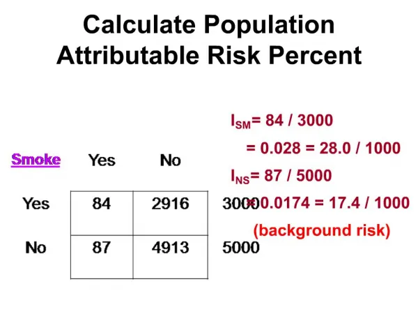
Example: Smoking, Cocaine Use, and Low Birthweight: Crude Associations Crude RR = 10.00 = 1.60 Crude RR = 30.00 = 4.77 6.25 6.29
Smoking and Cocaine Organized into a Risk System If smoking and cocaine use were recoded as a single “substance use” variable:
Component PAFs and Summary PAF for the Smoking-Cocaine Risk System Using Rothman’s formula: The Summary PAF is the sum of component PAFs + + + = 0.16
Limitation of Component PAFs from the Smoking-Cocaine Risk System While the component PAFs of a risk system sum to the Summary PAF for the system as a whole, they do not provide mutually exclusive measures of the PAF for each risk factor Here, the Summary PAF = 0.16, but the two factors overlap: the component PAFs still do not disentangle smoking and cocaine for those who do both Coc Sm/Coc Sm
The “Adjusted” PAF: Obtaining a Single PAF for a Given Risk Factor The Stratified Approach: The PAF for eliminating a risk factor after controlling for other risk factors With the Rothman formula, data are organized into the more traditional strata set-up for adjustment: Not assuming homogeneity, pj & RRj are stratum-specific: Assuming homogeneity, Overall
The “Adjusted” PAF: Obtaining a Single PAF for a Given Factor Reorganizing the data to get an adjusted PAF with Rothman’s formula
The “Adjusted” PAF: The PAF for Smoking, Controlling for Cocaine Use* RR=1.37 + = RR=1.36 *Using stratum-specific estimates
The “Adjusted” PAF:The PAF for Cocaine Controlling for Smoking* RR=4.33 + = RR=4.30 *Using stratum-specific estimates
Limitations of the “Adjusted” PAF: The resulting adjusted PAFs still are not mutually exclusive and they do not meet the criterion of summing to the Summary PAF for all factors combined ≠ 0.042+0.062+0.056=0.16 0.076 + 0.099 = 0.175
Sequential PAFs (PAFSEQ) for theSmoking-Cocaine Risk System For the smoking-cocaine risk system, there are 2 possible sequences: • Eliminate smoking first (a), controlling for cocaine use, then eliminate cocaine use (b) • Eliminate cocaine use first (a), controlling for smoking, then eliminate smoking (b) And within each sequence, there are two sequential PAFs
Sequential PAFs (PAFSEQ) for theSmoking-Cocaine Risk System • The 1st sequential PAF for eliminating smoking first, controlling for cocaine use (the “adjusted” PAF): PAFSEQ1a (S|C) = 0.076 • The 2nd sequential PAF for eliminating cocaine use after smoking has already been eliminated is the remainder of the Summary PAF PAFSEQ1b = PAFSUM – PAFSEQ1a (S|C) = 0.16 – 0.076 = 0.084
Sequential PAFs (PAFSEQ) for theSmoking-Cocaine Risk System • The 1st sequential PAF for eliminating cocaine use first, controlling for smoking (the “adjusted” PAF: PAFSEQ2a (C|S) = 0.099 • The 2nd PAF for eliminating smoking after cocaine use has already been eliminated is the remainder of the Summary PAF PAFSEQ2b = PAFSUM – PAFSEQ2a (C|S) = 0.16 – 0.099 = 0.061
Sequential PAFs (PAFSEQ) for theSmoking-Cocaine Risk System By definition, the sequential PAFs within the two possible sequences sum to the Summary PAF, but they still do not provide single measures of the impact of smoking or cocaine use regardless of the order in which they are eliminated Smoking First Cocaine Use First 0.076 + 0.084 = 0.16 0.099 + 0.061 = 0.16
Average PAF (PAFAVG) for theSmoking-Cocaine Risk System To obtain a single estimate, the sequential PAFs are rearranged, grouping the two for smoking together and the two for cocaine together and then calculating an average for each factor: • Eliminating smoking first, averaged with eliminating smoking second • Eliminating cocaine use first, averaged with eliminating cocaine use second
Average PAF (PAFAVG) for theSmoking-Cocaine Risk System Averaging Sequential PAFs Average PAF for Smoking: = Average PAF for Cocaine Use: =
Average PAFs for theSmoking-Cocaine Risk System The Average PAFs for each factor in the risk system are mutually exclusive and their sum equals the Summary PAF: 0.0685 + 0.0915 = 0.16
Model Building Issues and Strategies in the Context of Estimating and Reporting PAFs
Modeling to Generate AvgPAFs • Regression modeling is a flexible and efficient method for obtaining the series of relative risks needed for calculating seqPAFs as the number of variables being considered increases. • As an intermediate step in estimating avgPAFs, the modeling process will differ from that for estimating ratio measures of association: • Variable selection and organization • Level of Measurement & choice of reference groups • Confounding and effect modification • Model building strategies for choosing a final model
Variable Selection and Organization Classifying factors as modifiable or unmodifiable • When modeling to estimate relative risks or odds ratios, explicit differentiation between modifiable and unmodifiable factors is not necessary, although this differentiation is certainly conceptually important. • When modeling is an intermediate step in estimating avgPAFs, the question of modifiability must be tackled from the start, since variable handling proceeds differently according to how variables are classified.
Variable Selection and Organization Classifying factors as modifiable or unmodifiable • Unmodifiable factors are only used as potential confounders or effect modifiers; PAFs not calculated • Modifiable factors are factors that can possibly be altered with clear intervention strategies; these are the factors in the “risk system” • Being in the pool of modifiable factors not only influences final PAF estimates, but also may change choices about level of measurement, reference level, and handling of confounding and effect modification
Variable Selection and Organization Classifying factors as modifiable or unmodifiable Both broad and narrow definitions of modifiability may be reasonable, with some researchers computationally treating allvariables as modifiable, including factors such as race/ethnicity, age, and poverty; others treat as modifiable only factors that reflect a much narrower perspective on modifiability How close should the connection be between classification as modifiable and public health interventions?
Level of Measurement and Reference Groups • For unmodifiable factors, decisions about level of measurement, categorization schemes, and choice of reference groups can be made with the same considerations relevant to any epidemiologic modeling process. • For modifiable factors for which avgPAFs will be computed, however, level of measurement is constrained since avgPAFs are discrete measures anchored to levels, or categories, of exposure.
Level of Measurement and Reference Groups • Modifiable factors are in effect treated as dichotomous, comparing “any” to “no” risk. This mirrors the interpretation of a PAF as the proportion of disease reduction given complete elimination of exposure. • Defining the reference group as “lower risk” rather than “no” risk is one way to pull back from reporting an unrealistic maximum impact. For example: >= 2 days exercise, rather than >= 5 days exercise <=1 medical risk factor rather than 0 medical risks
Level of Measurement and Reference Groups Continuous or ordinal variable: • the “j” relative risks will be exponentiated multiples of a beta coefficient for each observed value. • the “unexposed”, or reference group, will include only those with the single lowest value of the variable; conversely, those with any other value will be considered “exposed” • With the single lowest value as the reference group, the proportion of exposed will likely be artificially high (an ordinal variable with a few levels will typically have a broader (more inclusive) reference group)
Level of Measurement and Reference Groups Dummy variables— whether a recoded continuous or ordinal variable or a nominal variable with k categories: • the “j” relative risks are computed from separate beta coefficients corresponding to the k-1 categories • for the special case of dichotomous variables, a single relative risk is computed from a single beta coefficient
Level of Measurement and Reference Groups • With dummy variables, the analyst can choose between reporting category-specific avgPAFs or an avgPAF for the summation over all categories. Note that while it is not possible to obtain a single ratio measure for a set of dummies, it is possible to obtain a single avgPAF. • If public health programming differs by exposure category, then using dummy variables and reporting dummy-specific avgPAFs may be more appropriate than summing over all categories.
Level of Measurement and Reference Groups Dummy variables may also be used to break up a single construct into modifiable and unmodifiable parts. Using prenatal care as an example, dummy variables might be:
Confounding and Effect Modification • For each modifiable factor, confounding by all other modifiable and unmodifiable factors should be assessed. This is no different than assessment of confounding in any model when precise estimation of multiple “exposures” is of interest • Accounting for effect modification, however, is related to whether it is present within the pool of unmodifiable factors, across modifiable and unmodifiable factors, or within the pool of modifiable factors